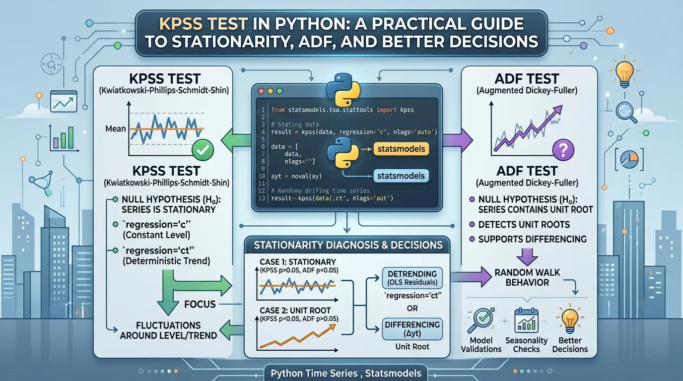

A time series can look calm and still fail a stationarity test. It can also rise steadily and remain stationary around a deterministic trend. That is why a single visual inspection, or a single p-value, rarely gives you enough information to decide how to transform data before forecasting.
The Kwiatkowski–Phillips–Schmidt–Shin (KPSS) test gives you one side of that diagnosis. Its null hypothesis is that the series is stationary around a constant or a deterministic trend. The Augmented Dickey–Fuller (ADF) test starts from the opposite position: its null hypothesis is that the series contains a unit root.
Used together, the tests create a useful diagnostic conversation. They do not replace domain knowledge, plots, seasonal analysis, or model diagnostics, but they can help you avoid blindly differencing every series that looks non-stationary.
This guide shows how to run the KPSS test in Python with current statsmodels, interpret the output without overstating what the test proves, and choose a sensible next step when KPSS and ADF disagree.
Key Takeaways
Click any topic to expand or collapseKPSS tests stationarity as the null hypothesis.
A small p-value is evidence against the selected stationarity specification.
A p-value above your significance level means “fail to reject”.
It does not mean stationarity has been proven.
Select the correct regression parameter carefully:
Use regression='c' for stationarity around a constant and regression='ct' for stationarity around a deterministic trend.
Run KPSS and ADF as complementary diagnostics.
Always inspect plots, seasonality, structural breaks, and model-specific assumptions alongside the tests.
Do not treat detrending and differencing as interchangeable.
Each operation addresses a different type of non-stationarity (trend-stationary vs. difference-stationary).
Best practices in current statsmodels implementation:
Prefer result_object=True for new code and always report the selected lag rule.
What does the KPSS test measure?
The KPSS test asks whether a time series is consistent with being stationary around a specified deterministic component. In practical terms, it tests whether the series fluctuates around:
- a constant level, using
regression='c'; or - a constant plus a deterministic linear trend, using
regression='ct'.
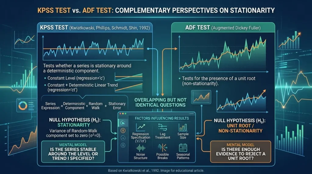
The original paper by [Kwiatkowski, Phillips, Schmidt, and Shin (1992)](https://doi.org/10.1016/0304-4076(92 )90104-Y) expresses the series as a combination of deterministic trend, random-walk behavior, and stationary error. The KPSS null sets the variance of the random-walk component to zero. That is the reason the test is commonly presented as a stationarity test with a null hypothesis opposite to ADF’s.
A useful mental model is this:
KPSS asks, “Is the series stable around the level or trend I specified?” ADF asks, “Is there enough evidence to reject a unit root?”
Those questions overlap, but they are not identical. The result depends on the regression specification, lag treatment, sample size, noise structure, and possible breaks or seasonal patterns.
Level stationarity vs. trend stationarity
Level stationarity
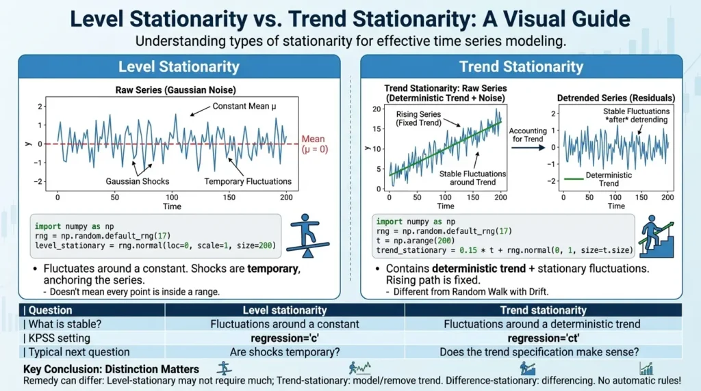
A level-stationary series fluctuates around a constant mean. Shocks may move the series temporarily, but the process tends to remain anchored around the same level.
A simple synthetic example is Gaussian noise centered near zero:
Python:
import numpy as np

rng = np.random.default_rng(17)
level_stationary = rng.normal(loc=0, scale=1, size=200)
This does not mean every observation must remain inside a fixed range. Stationarity is a property of the data-generating process, not a promise that the graph will never move sharply.
Trend stationarity
A trend-stationary series contains a deterministic trend plus stationary fluctuations. After accounting for that deterministic trend, the remaining deviations may be stable.
For example:
Python:
import numpy as np

rng = np.random.default_rng(17)
t = np.arange(200)
trend_stationary = 0.15 * t + rng.normal(0, 1, size=t.size)
The raw series rises, but that rise was generated by a fixed trend in this example. That is different from a random walk with drift, where shocks accumulate and permanently shift the path.
The distinction matters because the remedy can differ. A trend-stationary series may call for modeling or removing the deterministic trend. A difference-stationary series may require differencing. Neither conclusion should be made from one automatic rule.
| Question | Level stationarity | Trend stationarity |
|---|---|---|
| What is stable? | Fluctuations around a constant | Fluctuations around a deterministic trend |
| KPSS setting | regression='c' | regression='ct' |
| Typical next question | Are shocks temporary? | Does the trend specification make sense? |
KPSS hypotheses and p-values
For a chosen regression specification, the hypotheses are:
- Null hypothesis, H₀: the series is stationary around the selected constant or trend.
- Alternative hypothesis, H₁: the series is not stationary under that specification; the test is commonly described as testing against a unit-root or difference-stationary alternative.
At a significance level of 0.05:
- If
p_value <= 0.05, reject H₀. The data provides evidence against stationarity under the selected specification. - If
p_value > 0.05, fail to reject H₀. The result is compatible with stationarity, but it does not prove that the series is stationary.
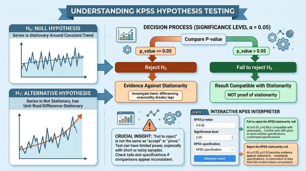
That second sentence is worth keeping visible in any production analysis. “Fail to reject” is not the same as “accept” or “prove.” A test can have limited power, especially with short or noisy samples, and a large sample can detect deviations that are statistically significant but practically small.
The test statistic and critical values tell the same story from another angle: reject the null when the statistic is more extreme than the critical value for the chosen significance level. When the p-value and critical-value comparison appear inconsistent, check that you are comparing the correct tail, specification, and significance level.
Interactive KPSS result interpreter
Use the interpreter below to translate a reported KPSS p-value into the correct statistical decision. It deliberately says “fail to reject” rather than “accept,” because a non-significant result is not proof of stationarity.
This tool interprets the decision rule only. It does not choose the correct regression specification, lag rule, transformation, or forecasting model.
How to run the KPSS test in Python
Install the main packages in your environment:
Bash:
python -m pip install numpy pandas matplotlib statsmodelsThe current statsmodels KPSS documentation documents regression, nlags, the result fields, p-value interpolation, and missing-value behavior. The examples below use the result-object form so the code names each output explicitly.
A modern reusable function
Python:
from __future__ import annotations

from typing import Any
import numpy as np
from statsmodels.tsa.stattools import kpss


def run_kpss(
    series: Any,
    *,
    regression: str = "c",
    nlags: str | int = "auto",
    alpha: float = 0.05,
) -> dict[str, Any]:
    """Run KPSS and return a labeled, JSON-friendly summary."""
    values = np.asarray(series, dtype=float)

    if values.ndim != 1:
        raise ValueError("series must be one-dimensional")
    if not np.isfinite(values).all():
        raise ValueError("series must not contain NaN or infinite values")
    if regression not in {"c", "ct"}:
        raise ValueError("regression must be 'c' or 'ct'")
    if not 0 < alpha < 1:
        raise ValueError("alpha must be between 0 and 1")

    result = kpss(
        values,
        regression=regression,
        nlags=nlags,
        result_object=True,
    )

    return {
        "statistic": float(result.statistic),
        "pvalue": float(result.pvalue),
        "lags": int(result.lags),
        "critical_values": {
            str(key): float(value)
            for key, value in result.critical_values.items()
        },
        "alpha": alpha,
        "decision": (
            "reject_stationarity_null"
            if result.pvalue <= alpha
            else "fail_to_reject_stationarity_null"
        ),
        "regression": regression,
        "nlags": nlags,
    }
Example usage:
Python:
level_result = run_kpss(level_stationary, regression="c")
trend_result = run_kpss(trend_stationary, regression="ct")

print(level_result)
print(trend_result)
The validation used for this article ran the examples with statsmodels 0.15.0. Your exact statistic and p-value will change when the input data, sample length, random seed, missing-value handling, or lag rule changes.
What if you need the older tuple interface?
The older form remains common in tutorials:
Python:
statistic, p_value, lags, critical_values = kpss(
    level_stationary,
    regression="c",
    nlags="auto",
    result_object=False,
)
It is useful when maintaining older code, but new code is easier to read when it uses named result attributes. The current documentation describes the default tuple-returning behavior as deprecated and documents a future change toward KPSSResult. Pin and record your statsmodels version when publishing a notebook or tutorial.
Choosing regression='c' or regression='ct'
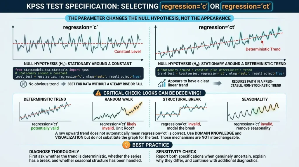
The parameter is not a cosmetic option. It changes the null hypothesis.
Python:
from statsmodels.tsa.stattools import kpss

# Stationary around a constant
level_test = kpss(series, regression="c", nlags="auto", result_object=True)

# Stationary around a constant plus deterministic trend
trend_test = kpss(series, regression="ct", nlags="auto", result_object=True)
Use domain knowledge and visualization to choose a plausible specification, but do not use the graph as a substitute for the test. A steadily rising graph can come from a deterministic trend, a random walk, a structural break, or seasonality. Those mechanisms are not interchangeable.
A useful sensitivity check is to report both specifications when the choice is genuinely uncertain, explain why they differ, and continue with additional diagnostics rather than selecting the result that supports a preferred model.
regression='ct' is correct. First ask whether the trend is deterministic, whether the series has a break, and whether seasonal structure has been handled.Understanding KPSS output, warnings, and lags
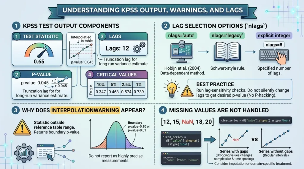
A KPSS result includes:
statistic: the test statistic;pvalue: a p-value interpolated from the KPSS reference table;lags: the truncation lag used for the long-run variance estimate; andcritical_values: critical values at 10%, 5%, 2.5%, and 1%.
With nlags='auto', statsmodels uses a data-dependent method associated with Hobijn et al. With nlags='legacy', it uses the Schwert-style rule documented in the API. An explicit integer is also possible:
Python:
result = kpss(
    series,
    regression="c",
    nlags=8,
    result_object=True,
)
There is no universally correct lag count for every dataset. For a sensitive analysis, run a small lag-sensitivity check and report whether the conclusion changes. Do not silently change lags until the p-value tells the story you want.
Why does InterpolationWarning appear?
statsmodels states that KPSS p-values are interpolated from the table in the original KPSS reference. If the computed statistic falls outside the table's range, the library returns a boundary p-value and warns that the true p-value is beyond that boundary.
For example, a displayed pvalue=0.10 can mean the actual p-value is greater than 0.10. A displayed pvalue=0.01 can mean the actual p-value is smaller than 0.01. Do not report those boundary values as highly precise measurements.
Missing values are not handled automatically
The official API documents that missing values are not handled. Clean or explicitly handle missing observations before calling kpss:
Python:
clean_series = df["value"].dropna().astype(float)
result = kpss(clean_series, regression="c", nlags="auto", result_object=True)
Dropping values can change the time spacing and sample size. If the series is sampled at regular intervals, document what happened and consider whether imputation or a domain-specific missing-data treatment is more appropriate.
KPSS vs. ADF: why use both?
The statsmodels ADF documentation defines ADF as a unit-root test for a univariate process in the presence of serial correlation. Its null hypothesis is that the series has a unit root; its alternative is that the series does not.
| Feature | KPSS | ADF |
|---|---|---|
| Null hypothesis | Stationary around the selected constant/trend | Unit root is present |
| Small p-value suggests | Evidence against stationarity | Evidence against a unit root |
| Main modeling question | Is the selected level/trend adequate? | Is a unit-root process plausible? |
| Best practice | Interpret with ADF and diagnostics | Interpret with KPSS and diagnostics |
The combination is informative because the null hypotheses point in opposite directions. But the tests can disagree for legitimate reasons: low power, near-stationarity, different deterministic terms, lag choices, serial correlation, structural breaks, or seasonal behavior.
A careful four-outcome guide
| KPSS result | ADF result | What it suggests | What to do next |
|---|---|---|---|
| Fail to reject stationarity | Reject unit-root null | Evidence consistent with stationarity | Check plots, residual behavior, seasonality, and model assumptions |
| Reject stationarity | Fail to reject unit-root null | Evidence consistent with non-stationarity | Investigate differencing, breaks, trend, and seasonal structure |
| Fail to reject stationarity | Fail to reject unit-root null | Inconclusive or low-power combination | Check sample size, specifications, lags, and additional tests |
| Reject stationarity | Reject unit-root null | Conflicting evidence | Review deterministic terms, breaks, lag choices, and data quality |
Some tutorials label the two conflict cases as “trend stationary” and “difference stationary.” That can be a useful hypothesis, but it is not an automatic classification. Use those labels as starting points for investigation, not as a machine-generated verdict.
The official statsmodels ADF/KPSS example demonstrates the complementary workflow and shows why a series should be tested again after a transformation.
Detrending is not the same as differencing
These operations answer different questions.
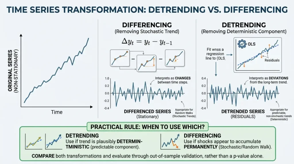
Differencing
First differencing transforms a series as:
In Python:
Python:
differenced = df["value"].diff().dropna()Differencing can remove a stochastic trend, but it also changes the interpretation of the series and can remove long-run information. It should be justified by the data and the model, not applied automatically because an ADF p-value is large.
Detrending
Detrending removes an estimated deterministic component, often by fitting a regression on time and analyzing the residuals:
Python:
import numpy as np
import statsmodels.api as sm

values = df["value"].dropna().to_numpy(dtype=float)
t = np.arange(values.size)
X = sm.add_constant(t)
trend_model = sm.OLS(values, X).fit()
detrended = trend_model.resid
The fitted trend is an estimate, not a known truth. A nonlinear trend, break, changing variance, or seasonality can make a simple linear detrending model inadequate. After transforming a series, rerun the relevant diagnostics and inspect whether the result makes sense in the original domain.
What KPSS does not tell you
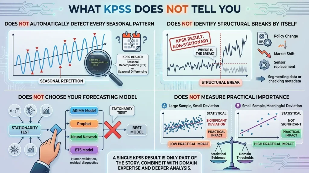
KPSS is useful, but it is not a complete time-series diagnostic.
It does not automatically detect every seasonal pattern
A series can have stable seasonal behavior and still fail a basic stationarity test if the seasonal component was not modeled. Consider seasonal plots, seasonal decomposition, seasonal differencing, or a model that represents the seasonal structure when the sampling frequency supports it.
It does not identify structural breaks by itself
A sudden policy change, measurement change, market regime shift, or sensor replacement can make a stable process look non-stationary. A single KPSS result cannot tell you whether a failure came from a unit root or a break. Segmenting the data, checking metadata, and using tests designed for breaks may be appropriate.
It does not choose your forecasting model
Stationarity testing is one input into model design. You still need time-aware validation, residual diagnostics, leakage checks, and a model specification suited to the target and forecast horizon.
It does not measure practical importance
With enough observations, a test may detect a small deviation from the null that has little operational impact. With too few observations, a meaningful deviation may remain undetected. Pair statistical evidence with domain thresholds and forecast performance.
A repeatable KPSS workflow
Use this checklist when you need a defensible stationarity decision:
- Confirm the time index: Sort observations, inspect the frequency, and check for duplicate or missing timestamps.
- Plot the raw series: Look for trend, seasonality, changing variance, outliers, and abrupt level shifts.
- Define the question: Are you testing level stationarity, trend stationarity, or the behavior after a transformation?
- Clean the input explicitly: Handle missing and non-finite values; document the decision.
- Run KPSS: Record
regression,nlags, statistic, p-value, lags, and critical values. - Run ADF: Record its regression specification and lag-selection method as well.
- Compare the tests cautiously: Treat disagreement as a diagnostic signal, not a shortcut to a label.
- Investigate seasonality and breaks: Do not attribute every failure to a unit root.
- Transform only when justified: Choose detrending, differencing, seasonal adjustment, or another approach based on the data-generating story.
- Re-test and validate: Run diagnostics again and evaluate the final forecasting workflow with time-aware validation.
The result should be a documented decision, not just a screenshot of one p-value.
Common mistakes to avoid
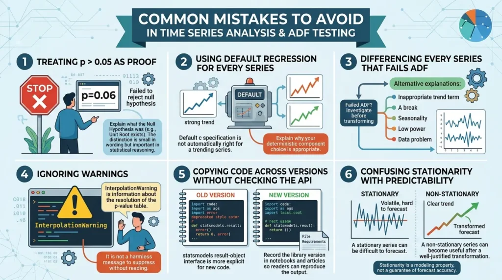
Mistake 1: Treating p > 0.05 as proof
Write “failed to reject the null” and explain what the null was. The distinction is small in wording but important in statistical reasoning.
Mistake 2: Using the default regression for every series
The default c specification is not automatically right for a trending series. Explain why your deterministic component is appropriate.
Mistake 3: Differencing every series that fails ADF
A failed ADF test can be consistent with a unit root, but it can also reflect an inappropriate trend term, a break, seasonality, low power, or a data problem. Investigate before transforming.
Mistake 4: Ignoring warnings
An InterpolationWarning is information about the resolution of the p-value table. It is not a harmless message to suppress without reading.
Mistake 5: Copying code across versions without checking the API
The statsmodels result-object interface is more explicit for new code. Record the library version in notebooks and articles so readers can reproduce the output.
Mistake 6: Confusing stationarity with predictability
A stationary series can be difficult to forecast. A non-stationary series can become useful after a well-justified transformation. Stationarity is a modeling property, not a guarantee of forecast accuracy.
Frequently asked questions
What is the null hypothesis of the KPSS test?
The KPSS null hypothesis is that the series is stationary around the selected deterministic component: a constant with regression='c', or a constant plus trend with regression='ct'.
How do I interpret a KPSS p-value below 0.05?
At a 0.05 significance level, a p-value below or equal to 0.05 is evidence against the KPSS stationarity null under the selected regression and lag specification. It does not identify the cause automatically.
What does a KPSS p-value above 0.05 mean?
It means you fail to reject the stationarity null at that significance level. The result is compatible with stationarity, but it is not proof that the series is stationary.
Should I use KPSS or ADF?
They answer complementary questions, so many workflows use both. Compare their results with plots, deterministic-term choices, lag settings, sample-size limitations, seasonality, and possible structural breaks.
What is the difference between regression='c' and regression='ct'?
regression='c' tests stationarity around a constant. regression='ct' includes a constant and deterministic linear trend in the stationarity specification.
Why does statsmodels show an InterpolationWarning?
KPSS p-values are interpolated from a reference table. When the statistic is outside the table range, statsmodels returns a boundary p-value and warns that the actual p-value is beyond that boundary.
Is differencing the same as detrending?
No. Differencing subtracts adjacent observations, while detrending removes an estimated deterministic trend. They can produce different transformed series and should be selected for different data-generating explanations.
Can KPSS detect structural breaks or seasonality?
KPSS alone cannot reliably identify whether a rejection comes from a unit root, a structural break, or unmodeled seasonality. Inspect the data and use diagnostics suited to those possibilities.
📋 Article Timeline & History
Successfully updated on September 10, 2026 with the latest details.
This article was originally published on September 8, 2026.

Was this article helpful?