
ARIMAX dynamic regression combines explanatory variables with an ARIMA error model. It can use information that a univariate forecast lacks: working days, scheduled promotions, temperature, or changes in income. But adding a useful historical predictor does not automatically create a useful forecasting model.
The missing step is usually a practical one: what value of that predictor will be available when the forecast is made? Tomorrow’s holiday status is known. Tomorrow’s temperature is a forecast. Next month’s revised economic indicator may not exist yet. Those inputs belong to different forecasting problems, even if they occupy adjacent columns in the same training matrix.
There is a second complication. “ARIMAX” does not name one universally agreed equation. Regression with ARIMA errors, ARX/ARMAX models, and transfer-function models represent dynamics differently. Software names can conceal those differences, especially when interpreting coefficients or specifying predictor lags.
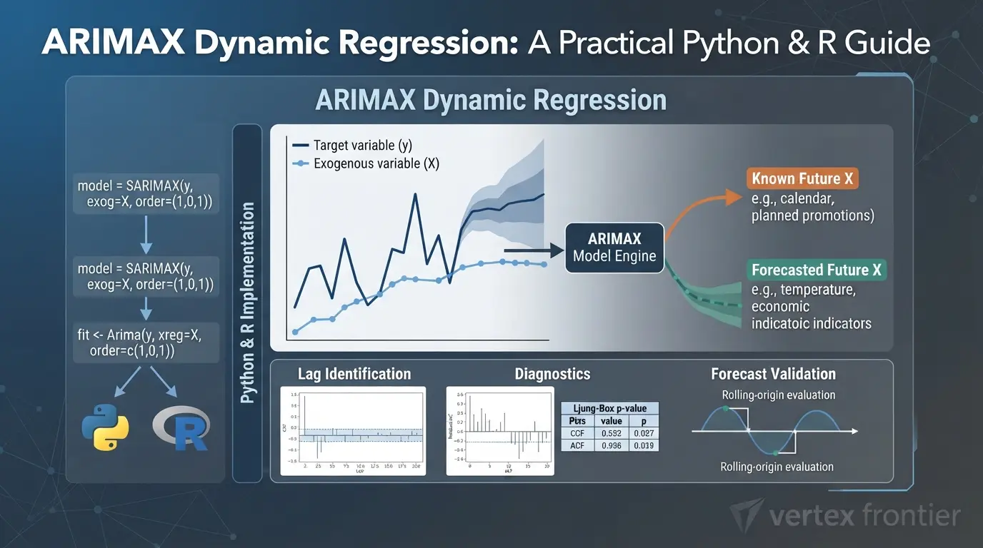
This guide starts with the model equation, then works through predictor availability, differencing, lag identification, Python and R implementation, diagnostics, and realistic validation. The organizing rule is the Covariate Contract: every explanatory variable must have an explicit source, timing rule, future-value policy, and fallback before it earns a place in the forecast.
Key takeaways
Click any topic to expand or collapseDeclare the equation and package
The ARIMAX label alone is not enough.
Separate known future inputs
Separate known future inputs from forecasts, scenarios, and unavailable inputs.
Use prewhitened cross-correlations
Use prewhitened cross-correlations to suggest lags—not to prove causality.
Set Ljung-Box degrees of freedom explicitly
A non-rejection is not a certificate.
Judge the complete forecasting pipeline
Judge the complete forecasting pipeline using only information available at each forecast origin.
Before you fit: five gates that prevent most ARIMAX mistakes
Run these checks before searching over ARIMA orders or adding more predictors:
- Target gate: define exactly what is being forecast, its time zone, aggregation, units, and whether the observed target is censored by stockouts, missing periods, or operational limits.
- Scale gate: decide whether the relationship is modeled in levels, logs, rates, or differences. Record every transformation and its inverse before fitting.
- Covariate gate: assign every X variable a Covariate Contract category, known, lagged, separately forecast, scenario-based, or unavailable, and state who supplies it at forecast time.
- Baseline gate: fit a naive or seasonal-naive benchmark and a univariate ARIMA/SARIMA baseline under the same forecast horizon.
- Validation gate: choose forecast origins, horizon, refitting policy, metrics, and interval checks before inspecting the final test period.
If any gate has no defensible answer, stop model tuning and resolve the data or forecasting-information problem first. A more complicated ARIMAX specification cannot repair an undefined target or an unavailable future input.
What is ARIMAX, and how does it differ from ARIMA?
ARIMAX is an ARIMA-related forecasting model that includes external regressors. In the regression-with-ARIMA-errors formulation used throughout most of this guide, the regression describes the relationship between predictors and the response.
The ARIMA process describes the remaining serial dependence.
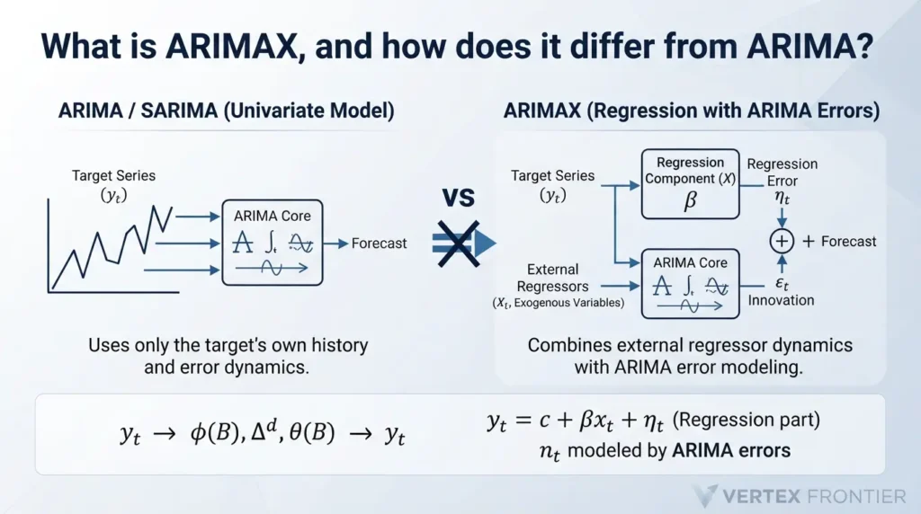
ARIMA uses the target’s own history and error dynamics without an external predictor matrix. SARIMA adds seasonal dynamics. ARIMAX adds regressors; SARIMAX combines seasonal ARIMA errors with regressors in common software usage. The Python class named SARIMAX can also fit non-seasonal models by leaving its seasonal component inactive.
If you need the underlying AR, integration, and MA concepts first, the ARIMA time-series forecasting guide explains the univariate baseline. That baseline remains important: ARIMAX should have to beat it under the same forecasting conditions.
The FPP3 chapter on dynamic regression makes a crucial distinction between two errors:
- Regression error, η: the part of the response not explained by the regressors. It may be autocorrelated.
- Innovation, ε: the new disturbance left after the ARIMA structure has accounted for predictable dependence. This is the series modeled as white noise.
A regression error with a strong ACF is not necessarily a problem. A strong ACF in the fitted innovation residuals is more concerning. Confusing the two can lead you to “repair” a model whose error structure is doing exactly what it was designed to do.
Four structures hidden behind similar names
Hyndman’s explanation of the ARIMAX naming problem distinguishes regression with ARMA errors from ARMAX and more general transfer functions. The same distinctions extend to integrated and seasonal models, but naming varies across books and packages.
In the table, B is the backshift operator: it moves a series back one observation. The AR and MA polynomials are φ and θ; Δ denotes differencing. Constants and seasonal terms must be specified separately when required. The displayed ARX/ARMAX example is stationary, with one contemporaneous input.
| Structure | Representation | How X enters | Implementation boundary |
|---|---|---|---|
| ARIMA / SARIMA | Target modeled using its own dynamics, with optional seasonal operators. | No external predictor matrix. | A necessary univariate comparator, not an inferior model by definition. |
| Regression with ARIMA errors | yt = c + Σ βjxj,t + ηt φ(B)Δdηt = θ(B)εt | Through the supplied regression columns, including any deliberately constructed lags. | forecast::Arima with xreg; fixed-regression statsmodels SARIMAX with exog, subject to trend and differencing options. |
| ARX / ARMAX | φ(B)yt = c + βxt + θ(B)εt | Alongside lagged response terms. Solving the stable recursion creates a distributed input response. | AutoReg is an AR-X implementation, not an arbitrary ARMAX or transfer-function estimator. |
| Transfer-function regression | yt = c + [ω(B)Bb/δ(B)]xt + ηt η has a separate ARIMA error model. | Through a delay b, numerator weights ω, and denominator dynamics δ. | TSA::arimax exposes transfer-filtered xtransf inputs as well as ordinary xreg covariates. |
A regression with ARIMA errors can include lagged X columns. It is not restricted to contemporaneous predictors. What it does not do automatically is estimate an arbitrary delayed, decaying transfer filter just because you supplied one X column.
Likewise, the autoregressive order of the error model does not mean “include that many lags of every predictor.” If an effect begins three periods later, construct the delayed input or use a transfer-function specification that encodes it.
Choose the statistical structure before choosing the function name.
What ARIMAX coefficients do, and do not mean
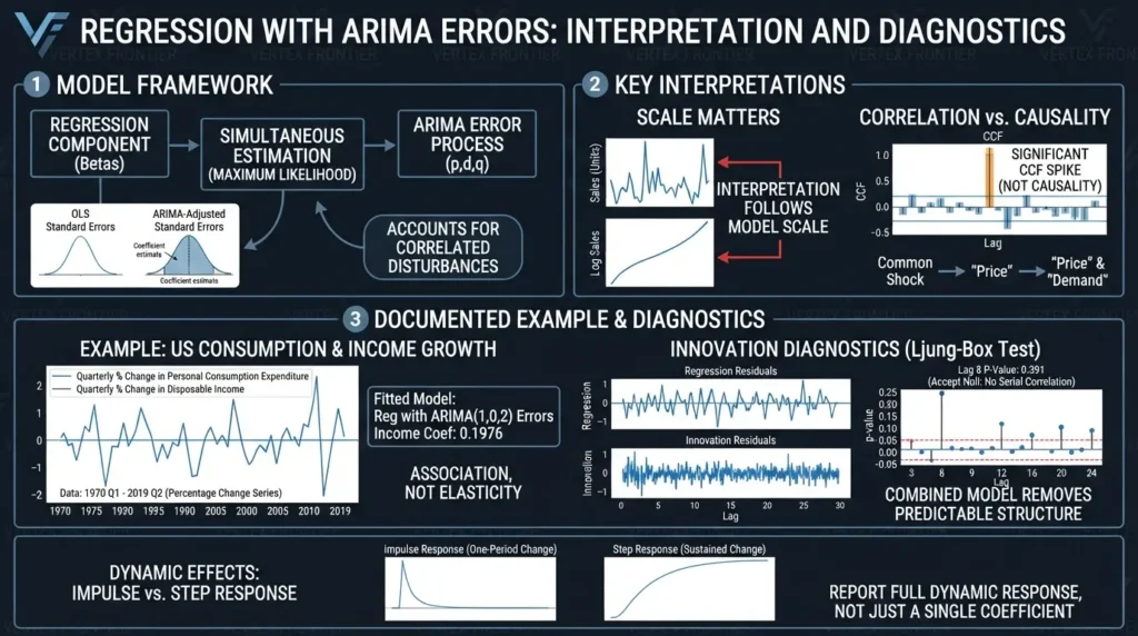
A regression slope describes a conditional association on the modeled scale, given the other included regressors and the specified error process. With ARIMA errors, estimation accounts for correlated disturbances; it is not ordinary iid OLS simply because the software documentation uses “OLS-type regressors.”
Penn State’s lesson on regression with ARIMA errors describes simultaneously estimating regression and error parameters by maximum likelihood. This differs from fitting iid OLS and treating its usual standard errors as appropriate for serially correlated disturbances.
The scale matters. A slope for sales in units is not a slope for log sales. A relationship between quarterly percentage changes is not a relationship between expenditure and income levels. Differencing changes the stationary representation used for estimation, so interpretation must follow the actual model, not the column’s business label.
Neither a positive coefficient nor a prewhitened CCF spike establishes causality. Price can respond to expected demand. Promotional spending can be increased when sales are weak. Common shocks can move both the predictor and the target. Calling a column “exogenous” does not remove these feedback or confounding problems.
For forecasting, ask whether the feature provides stable, available predictive information. For causal analysis, a separate identification design must address timing, confounding, and endogeneity. Adding ARIMA errors is not that design.
Documented example: US consumption and income
In the FPP3 US consumption and income example, the task is to forecast quarterly changes in personal consumption expenditure using changes in disposable income. The displayed data cover 1970 Q1 to 2019 Q2. These are percentage-change series, rather than trending expenditure and income levels.
The textbook fits a regression with ARIMA(1,0,2) errors and reports an income coefficient of 0.1976. On that model’s scale, an additional percentage point of quarterly income growth is associated with about 0.198 percentage points of consumption growth, conditional on the fitted specification. This is a published model estimate, not evidence of a causal income elasticity.
The source then separates regression residuals from innovation residuals. Its innovation diagnostic at lag eight uses three model degrees of freedom and reports a Ljung-Box p-value of 0.391. That illustrates how the regression can leave serially correlated errors while the combined model removes much of their predictable structure.
The outcome is a documented fitted model and diagnostic result, not a measured business improvement. The lesson is more useful than a generic “X improves accuracy” claim: define the scale, model the remaining dependence, and diagnose the innovations.
Dynamic effects remain interpretable
In a stable ARX or transfer-function model, the response to an input can unfold over several periods. A single coefficient does not summarize that whole response.
Report an impulse response for a one-period input change and a step response for a sustained input change. The former shows when the effect starts and how it decays; the latter shows how effects accumulate. A transfer-function denominator governs the input-response component, which is distinct from the separate ARIMA noise process.
Do not replace that denominator mechanically with a lagged response term. Algebraic rearrangements can also change the implied error equation. The full model is what must be estimated and interpreted.
The Covariate Contract: decide how every future X will exist
An exogenous variable is an external regressor supplied to the forecasting model rather than the response being forecast. In a statistical model, exogeneity also involves assumptions about its relationship to the disturbance. A software argument named exog or xreg does not verify those assumptions.
The Covariate Contract is a practical framework for making each input’s forecasting role explicit. Classify every predictor into one of five categories before fitting the model.
| Input category | Future-value policy | Validation requirement | Fallback |
|---|---|---|---|
| Known / planned | Generate calendars; use the promotion or operating plan recorded at the forecast origin. | Do not substitute the final executed plan for the earlier planned version. | Versioned revised plan or an explicitly defined no-event scenario. |
| Lagged | Use past measurements only while their lag and release delay cover the required horizon. | Check availability separately at every forecast step. | Shorten the horizon, forecast the remaining inputs, or use a reduced model. |
| Separately forecast | Obtain weather, economic, or other predictor forecasts from an upstream model or provider. | Use forecast vintages available then; assess predictor uncertainty. | Approved substitute forecast or a separately validated predictor-free model. |
| Scenario | Supply a deliberate assumption about prices, temperature, or another input. | Label the forecast conditional on that assumption; do not imply the scenario is predicted. | A reviewed set of plausible alternative paths. |
| Unavailable | No defensible future path exists at the required horizon. | Do not claim an operational forecast that depends on hindsight values. | Exclude it, change the task, or select another modeling design. |
For every row, record the data owner, refresh time, publication delay, revision policy, units, transformations, supported horizon, and response to missing values. A feature without a reliable contract is not production-ready merely because its coefficient is significant.
Lagged does not mean known forever. Suppose the model uses a predictor measured seven days earlier. With immediate reporting, its values for the first seven forecast days are already in the historical record. For days eight onward, new predictor values are still needed. A reporting delay shortens even that initial window.
Planned inputs need similar care. A final promotion calendar contains decisions that may have changed after a historical forecast was issued. Backtesting with that final calendar evaluates a better-informed system than the one that actually existed.
OTexts’ forecasting guidance states the underlying requirement plainly: future predictors must be known, modeled separately, or assigned assumed values. The contract turns that statistical requirement into an implementation decision.
Community discussions expose the same practical obstacle. In an r/statistics thread about forecasting beyond the last ARIMAX predictor, the author asks whether forecasting the predictors will compound uncertainty. This is community evidence of an implementation question, not a benchmark or a universal failure claim.
The forecasting horizon belongs in feature selection, not just in the final prediction call.
Before and after: change the workflow, not just the model
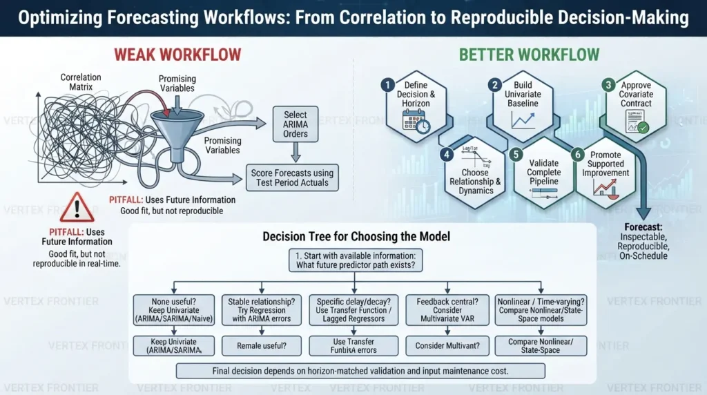
A weak workflow starts with a large correlation matrix, adds promising variables, selects ARIMA orders, and scores forecasts using the test period’s actual X values. It may produce a good fit without answering whether the same inputs could have been supplied in real time.
A better workflow reverses the order:
- Define the decision and horizon. Specify when forecasts are issued and what they support.
- Build a univariate baseline. Keep the naive or seasonal-naive comparator as well as ARIMA/SARIMA.
- Approve the Covariate Contract. Exclude features whose future-value policy does not match the task.
- Choose the relationship and dynamics. Decide on levels, changes, explicit lags, or a transfer response.
- Validate the complete pipeline. Recreate predictor availability, preprocessing, refitting, and forecasting at historical origins.
- Promote only a supported improvement. Preserve the baseline as a separately validated fallback.
The “after” result is not a promised accuracy gain. It is a forecast whose assumptions can be inspected, reproduced, and supplied on schedule.
A decision tree for choosing the model
Start with the information available, then choose the structure:
- No useful future predictor path? Keep a univariate model or shorten the horizon.
- Available predictors with a reasonably stable relationship? Try regression with ARIMA/SARIMA errors.
- A specific delay or decaying response matters? Compare explicit lagged regressors with a parsimonious transfer-function model.
- Predictors and target need joint forecasting because feedback is central? Consider a multivariate model, such as VAR, rather than treating every input as given.
- Relationships are nonlinear, change over time, or span many thin series? Compare nonlinear features, time-varying state-space models, or pooled supervised designs under the same information set.
These are candidate routes, not rankings. The final decision depends on horizon-matched validation and the cost of maintaining the inputs.
Stationarity and differencing: choose the relationship first
Do not automatically difference every X because Y is differenced. First decide what relationship the model represents, then check how the software implements that relationship.
The FPP2 explanation of regression with ARIMA errors shows that a levels regression with integrated errors has an equivalent representation in differenced variables. In forecast::Arima, specifying differencing applies the transformation to the regression variables during estimation. That is not a command to manually difference all inputs beforehand and then let the function difference them again.
Work through these cases:
- The response and predictors are stationary on the chosen scale. Fit without unnecessary differencing and model residual dependence.
- Nonstationary levels lack a defensible stable relationship. Consider a model in changes or other transformations. Shared trends alone can create misleading regression evidence.
- A long-run levels relationship is plausible. Investigate cointegration and an appropriate levels/error-correction specification instead of discarding that relationship by default.
- The response is integrated but an input is already stationary. Do not manually difference that input solely because of the response’s integration order. A model of changes in Y against levels of X is possible, but it is a different equation from a levels regression with integrated errors.
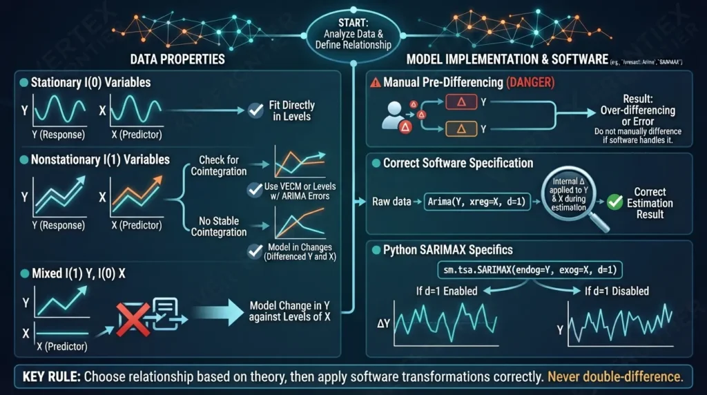
An I(0) stationary predictor and an I(1) response do not, by themselves, create a cointegration problem to solve. Cointegration concerns a stationary combination of nonstationary series. The relevant question is whether your chosen relationship and disturbance specification are defensible.
Use plots, domain knowledge, seasonal structure, and complementary stationarity tests. The practical KPSS and ADF guide explains their different null hypotheses. Neither test selects predictor lags, proves cointegration, or distinguishes every structural break from a stochastic trend.
Python has an additional boundary. The SARIMAX API documentation states that simple differencing transforms both endog and exog before state-space estimation. With that option enabled, predictions concern differenced data; with it disabled, the state-space model produces predictions on the original data scale.
Keep a written transformation specification. It should say what the response represents, which regressors enter, where differencing occurs, and how predictions return to the reporting scale.
Prewhitening and CCF: identify candidate lags, not causal facts
The cross-correlation function, or CCF, measures association between two series at different time offsets. It can suggest whether past values of an input may help predict the current response.
Raw CCF patterns can be hard to interpret when both series have autocorrelation, trends, or common seasonality. A broad collection of spikes may reflect those features rather than many separate delayed effects. Penn State’s prewhitening lesson presents prewhitening as an aid to identification, not as a universal requirement.
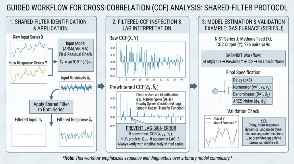
Step by step: the shared-filter protocol
- Align the series. Use a regular time index, consistent aggregation, and an explicit missing-data policy. Separate reporting time from observation time.
- Fit a parsimonious input model. Model X with suitable ARMA/ARIMA dynamics. Check whether its residuals are close enough to white noise for useful exploration; do not keep increasing orders merely to erase every spike.
- Apply the same estimated filter to Y. Include the same differencing and AR/MA filtering, with compatible initialization. Fitting an unrelated model to Y is not the classical shared-filter procedure.
- Inspect the filtered CCF. Treat candidate lags and response shapes as hypotheses. Account for edge losses and align the surviving observations.
- Fit candidate models to the original modeling data. Include the proposed lags or transfer structure, estimate the remaining error dynamics, and validate out of sample.
A narrow spike may suggest a delayed regressor. Several nearby spikes may suggest a finite distributed lag. A smooth decay may motivate a transfer denominator. An oscillating pattern can motivate a more complex response, but competing specifications may explain it too.
Approximate two-standard-error bands are only rough references. Filter estimation, finite samples, missing observations, and inspecting many lags affect interpretation. A spike outside the band is a reason to investigate, not proof of a genuine physical mechanism.
Prevent the lag-sign error
Write the intended relationship in words before reading the plot: X from three observations ago predicts Y now.
The official R CCF documentation defines its lag value using X at time t plus k against Y at time t. With X supplied first and Y second, the past-X relationship above appears at lag minus three, not plus three. Reversing the series reverses the sign. For ts objects, the axis is in time units, so frequency also matters.
The STAT 878 cross-correlation lecture emphasizes this variable-order problem. As teaching evidence, it reinforces a simple safeguard: verify a library’s convention with a deliberately shifted series before translating plot locations into lagged features.
Documented methodological example: the Box-Jenkins gas furnace
The classic Series J experiment measured methane feed rate and output CO₂ concentration. NIST documents 296 paired observations collected at nine-second intervals. Its own displayed analysis uses the first 60 pairs for a bivariate autoregressive model; that is not the same fit as the transfer-function example.
The SAS worked Series J analysis follows the input-output route: fit an AR(3) model to the input, prewhiten both series, examine cross-correlations, fit an initial transfer response, and then model the remaining noise.
Its final specification includes a three-observation delay, a numerator through lag two, a first-order transfer denominator, and separate AR(2) noise. The documented outcome is that fitted structure and its residual checks, not a single CCF spike or a published operational accuracy lift.
The lesson is the sequence. Delay, input-response dynamics, and noise dynamics are separate decisions. A contemporaneous X column plus an arbitrary ARIMA order is not a substitute for that sequence.
Use prewhitening to narrow a candidate set, then let estimation, diagnostics, stability, and forecasting tests decide.
The Python and R snippets below are illustrative workflows, not published benchmark results. Before production use, pin the Python/R runtime and package versions, run the complete script, record convergence and diagnostics, and keep the future-feature construction alongside the fitted model.
Do not infer that SARIMAX, forecast::Arima, and TSA::arimax have interchangeable defaults. Their parameterization, trend/intercept handling, differencing options, transfer conventions, and prediction interfaces must be checked in the exact release you deploy.
SARIMAX Python example: make the future-X contract visible
The example below uses synthetic daily observations with a smooth weekly pattern, a predetermined event schedule, and ARMA noise. Every future regressor is known by construction. This isolates the mechanics of fitting and forecasting without pretending that future weather or income has already been observed.
The Python data-library guide explains where Statsmodels fits alongside NumPy, Pandas, and other tools. Here, SARIMAX is used as a fixed-coefficient regression with ARMA errors; its seasonal error component is inactive because weekly structure is supplied as regression terms.
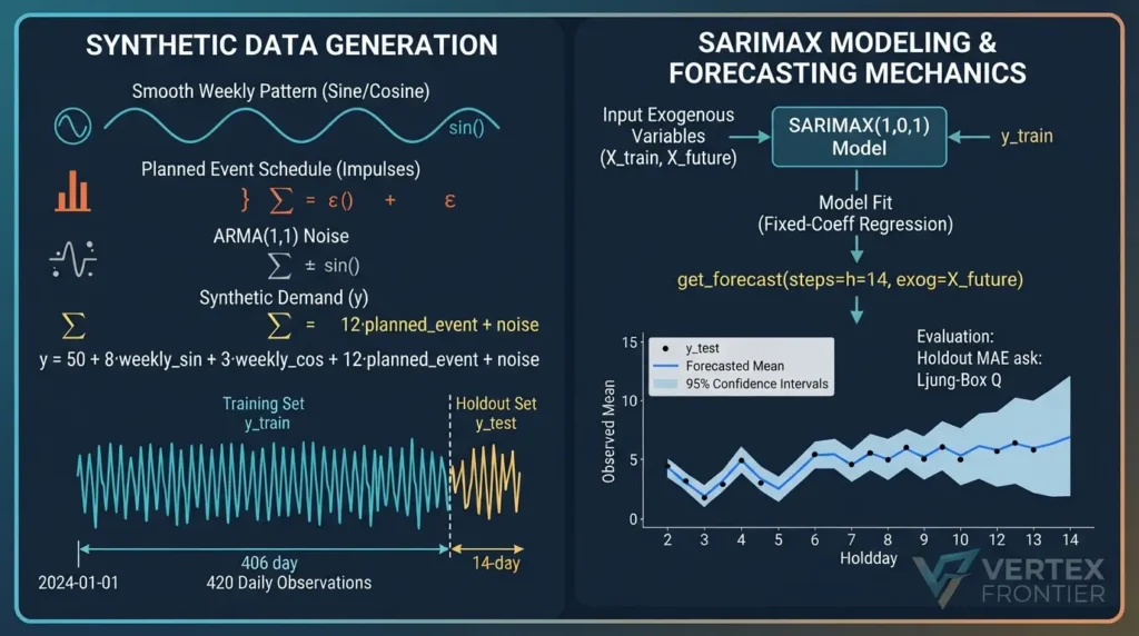
Validation note: this is illustrative code, not an executed benchmark or production template. Pin and test the Python runtime and package/API versions before production. The version printout records your environment; it does not specify a tested environment for this article.
Python — illustrative SARIMAX with known future regressors:
import sys
import numpy as np
import pandas as pd
import matplotlib.pyplot as plt
import statsmodels
from statsmodels.tsa.statespace.sarimax import SARIMAX
from statsmodels.stats.diagnostic import acorr_ljungbox
print("Python:", sys.version.split()[0])
print("NumPy:", np.__version__, "Pandas:", pd.__version__)
print("Statsmodels:", statsmodels.__version__)
rng = np.random.default_rng(42)
n, h = 420, 14
t = np.arange(n)
dates = pd.date_range("2024-01-01", periods=n, freq="D")
All columns depend only on the calendar or a fixed plan.
X = pd.DataFrame({
"const": np.ones(n),
"weekly_sin": np.sin(2 * np.pi * t / 7),
"weekly_cos": np.cos(2 * np.pi * t / 7),
"planned_event": (t % 84 < 3).astype(float),
}, index=dates)
Synthetic response: regression plus ARMA(1,1) disturbances.
eps = rng.normal(0, 2, n)
noise = np.zeros(n)
noise[0] = eps[0]
for i in range(1, n):
noise[i] = 0.55 * noise[i - 1] + eps[i] + 0.2 * eps[i - 1]
y = pd.Series(
50 + 8 * X["weekly_sin"] + 3 * X["weekly_cos"]
+ 12 * X["planned_event"] + noise,
index=dates, name="synthetic_demand",
)
y_train, y_test = y.iloc[:-h], y.iloc[-h:]
X_train, X_future = X.iloc[:-h].copy(), X.iloc[-h:].copy()
expected_index = pd.date_range(
y_train.index[-1] + pd.Timedelta(days=1), periods=h, freq="D"
)
assert X_train.index.equals(y_train.index)
assert X_future.index.equals(expected_index)
assert X_future.shape == (h, X_train.shape[1])
assert list(X_future.columns) == list(X_train.columns)
assert np.isfinite(X_train.to_numpy()).all()
assert np.isfinite(X_future.to_numpy()).all()
assert np.isfinite(y_train.to_numpy()).all()
model = SARIMAX(
y_train, exog=X_train, order=(1, 0, 1),
seasonal_order=(0, 0, 0, 0), trend="n",
time_varying_regression=False, mle_regression=True,
simple_differencing=False,
enforce_stationarity=True, enforce_invertibility=True,
)
result = model.fit(disp=False)
if not result.mle_retvals.get("converged", False):
raise RuntimeError("Fit did not converge; investigate before forecasting.")
prediction = result.get_forecast(steps=h, exog=X_future)
mean = prediction.predicted_mean
interval = prediction.conf_int(alpha=0.05)
output = pd.DataFrame({
"actual": y_test,
"forecast": mean,
"lower_95": interval.iloc[:, 0],
"upper_95": interval.iloc[:, 1],
})
print(output)
print("Holdout MAE:", np.mean(np.abs(y_test - mean)))
Non-seasonal ARMA(1,1) error convention: model_df = 2.
burn = int(result.loglikelihood_burn)
innovations = np.asarray(result.resid)[burn:]
innovations = innovations[np.isfinite(innovations)]
print(acorr_ljungbox(
innovations, lags=[7, 14], model_df=2, return_df=True
))
result.plot_diagnostics(figsize=(10, 8))
plt.show()
Several choices are deliberate. The constant is a regression column, while the separate trend is disabled. The Statsmodels SARIMAX/ARIMA FAQ explains why a trend intercept and a constant supplied through exog are not interchangeable parameter labels in every representation.
The ARMA order matches the synthetic design; it is not a recommended default for real demand. Likewise, the printed holdout error is a plumbing check, not evidence that this specification beats a baseline. Real model selection needs several historical origins and the deployment horizon.
Before adapting the example, verify:
- Rows: one future design row per forecast step.
- Columns: the same count, meaning, and order as at fitting time.
- Index: the expected timestamps, frequency, and aggregation boundaries.
- Transformations: the same training-fitted scaling, encoding, and feature construction.
- Missingness: an explicit handling policy, not an unnoticed NaN or filled future observation.
Use explicit exceptions rather than relying only on assertions in a deployed pipeline, where Python assertions can be disabled. Shape checks cannot detect a temperature column accidentally expressed in a different unit; semantic checks are part of the contract too.
ARIMAX in R: forecast::Arima and future xreg
The official forecast::Arima reference defines the fitted model as regression with ARIMA errors. Its xreg input is a numerical vector or matrix with one row per response observation; it should not be a data frame.
The following R example uses the same synthetic design as the Python example, but the random disturbances are generated independently. It is a parallel workflow, not a claim that the two languages produce identical data or estimates.
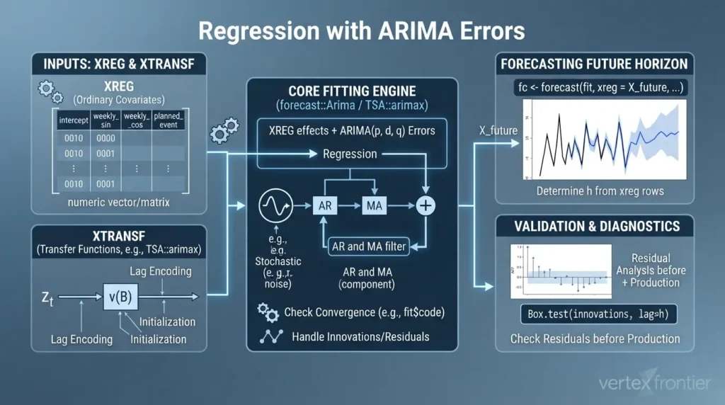
Validation note: the code is illustrative and has not been executed here. Pin and test R and the forecast package/API version before production. Check convergence, residual extraction, forecast methods, and version-specific behavior in that environment.
R — illustrative regression with ARIMA errors and future xreg:
library(forecast)
print(R.version.string)
print(packageVersion("forecast"))
set.seed(42)
n <- 420L
h <- 14L
t <- 0:(n - 1L)
X <- cbind(
const = rep(1, n),
weekly_sin = sin(2 * pi * t / 7),
weekly_cos = cos(2 * pi * t / 7),
planned_event = as.numeric(t %% 84 < 3)
)
noise <- as.numeric(arima.sim(
model = list(ar = 0.55, ma = 0.2), n = n, sd = 2
))
y <- ts(
50 + 8 * X[, "weekly_sin"] + 3 * X[, "weekly_cos"] +
12 * X[, "planned_event"] + noise,
frequency = 7
)
train_rows <- seq_len(n - h)
future_rows <- (n - h + 1L):n
y_train <- ts(as.numeric(y)[train_rows], frequency = 7)
y_test <- as.numeric(y)[future_rows]
X_train <- X[train_rows, , drop = FALSE]
X_future <- X[future_rows, , drop = FALSE]
stopifnot(
nrow(X_train) == length(y_train),
nrow(X_future) == h,
ncol(X_future) == ncol(X_train),
identical(colnames(X_future), colnames(X_train)),
all(is.finite(X_train)), all(is.finite(X_future)),
all(is.finite(y_train))
)
The constant is already supplied in X, so disable another mean.
fit <- Arima(
y_train, xreg = X_train, order = c(1, 0, 1),
include.mean = FALSE, include.drift = FALSE, method = "ML"
)
if (!is.null(fit$code) && fit$code != 0L) {
stop("Fit did not converge; investigate before forecasting.")
}
fc <- forecast(fit, xreg = X_future, h = h, level = 95)
print(coef(fit))
print(data.frame(
actual = y_test, forecast = as.numeric(fc$mean),
lower_95 = as.numeric(fc$lower[, 1]),
upper_95 = as.numeric(fc$upper[, 1])
))
print(mean(abs(y_test - as.numeric(fc$mean))))
innovations <- as.numeric(residuals(fit, type = "innovation"))
innovations <- innovations[is.finite(innovations)]
for (lag_h in c(7L, 14L)) {
print(Box.test(
innovations, lag = lag_h, type = "Ljung-Box", fitdf = 2L
))
}
acf(innovations, lag.max = 14)
plot(fc)
When future xreg is supplied, the forecast.Arima method uses its row count to determine the horizon. Do not assume an h argument repairs an incorrectly sized future matrix. Maintain your own checks for column order, transformations, and timestamp alignment.
For real data, keep dates alongside the numeric design matrix. A ts frequency expresses regular spacing and seasonality; it does not establish that a particular row is the correct holiday, billing day, or publication vintage.
You can use auto.arima to select the ARIMA error structure for a supplied predictor set. It does not discover all appropriate predictors or their lag structures for you. Compare a restrained set of feature designs, and perform selection inside the training portion of each validation fold.
Where TSA::arimax fits
The official TSA::arimax help separates ordinary xreg covariates from xtransf covariates whose effects pass through transfer filters. The transfer argument specifies those filters; the function also exposes fixed coefficients and initialization options.
For distributed-lag xtransf inputs, the help notes that the filter starts with zero initial values and that mean deletion is pertinent and not automatic. This is an initialization warning for those filtered covariates, not a universal instruction to center every exogenous variable.
Before building a transfer example, check the exact delay encoding, numerator convention, parameter ordering, initial conditions, and prediction procedure against the TSA implementation source for the pinned release. Transfer-order conventions are not safely inferred from another package’s ARMA notation. Fitting machinery is only one part of identification, estimation, and validation.
Seasonal ARIMAX, SARIMAX, and long seasonality
Seasonality can enter through the regression mean, the error process, or both. These choices answer different questions.
Calendar regressors explain known patterns such as working days or a moving holiday. Seasonal ARIMA errors describe dependence that remains at seasonal lags. A model with calendar terms may still need seasonal errors; a seasonal error model does not automatically encode the exact dates of a moving event.
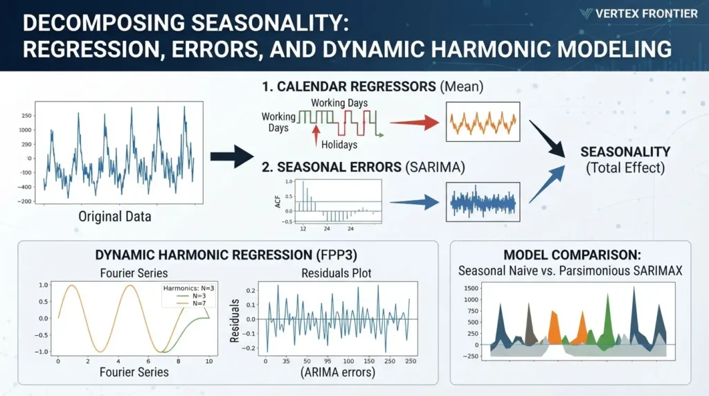
For a regular monthly series, compare a seasonal-naive baseline and a parsimonious SARIMA/SARIMAX specification. Check whether sufficient seasonal cycles remain after holding out data, adding lags, and differencing. There is no universal observation-count threshold that guarantees reliable seasonal estimation.
For long or multiple seasonal periods, dynamic harmonic regression in FPP3 uses Fourier terms to represent smooth seasonal patterns and ARIMA errors for remaining short-term dependence. Fourier regressors are known into the future once their periods and calendar alignment are defined.
Use that route when a smooth repeating shape is plausible. It is not automatically preferable for abrupt holiday effects, evolving seasonal patterns, or operational calendars that do not repeat at a fixed interval. Choose the number of harmonics inside validation; too many can fit noise or compete with other seasonal terms.
A practical sequence is to model known calendar effects, inspect the remaining seasonal dependence, and compare seasonal errors against harmonic alternatives. Avoid adding a large seasonal feature set and a large seasonal ARIMA component merely because both are available.
Separate predictable calendar structure from seasonal dependence left in the errors.
Ljung-Box diagnostics: use model_df, not a universal shortcut
The Ljung-Box test assesses a group of residual autocorrelations through a chosen maximum lag. Its p-value relies on a reference distribution and an adjustment for fitted-model degrees of freedom. It does not test every aspect of forecast quality.
Statsmodels’ acorr_ljungbox documentation exposes that adjustment as model_df. The selected lag minus model_df supplies the reference degrees of freedom; if the result is nonpositive, the function returns NaN for the p-value.
For a conventional non-seasonal ARMA error model, counting estimated AR and MA coefficients is a common asymptotic convention. The illustrative code therefore uses two for its ARMA(1,1) errors. It does not subtract every regression coefficient or the variance parameter.
Hyndman’s investigation of Ljung-Box degrees of freedom supports counting ARMA coefficients for regression with ARMA errors in the simulations considered. It also finds that seasonal-model calibration is less straightforward than counting every parameter.
Those empirical findings do not establish one adjustment for all seasonal, transfer-function, or state-space models.
In R, Box.test exposes the corresponding adjustment as fitdf. In Python, specifying a seasonal period in acorr_ljungbox changes its default lag selection; it does not automatically decide the right model_df for your fitted model.
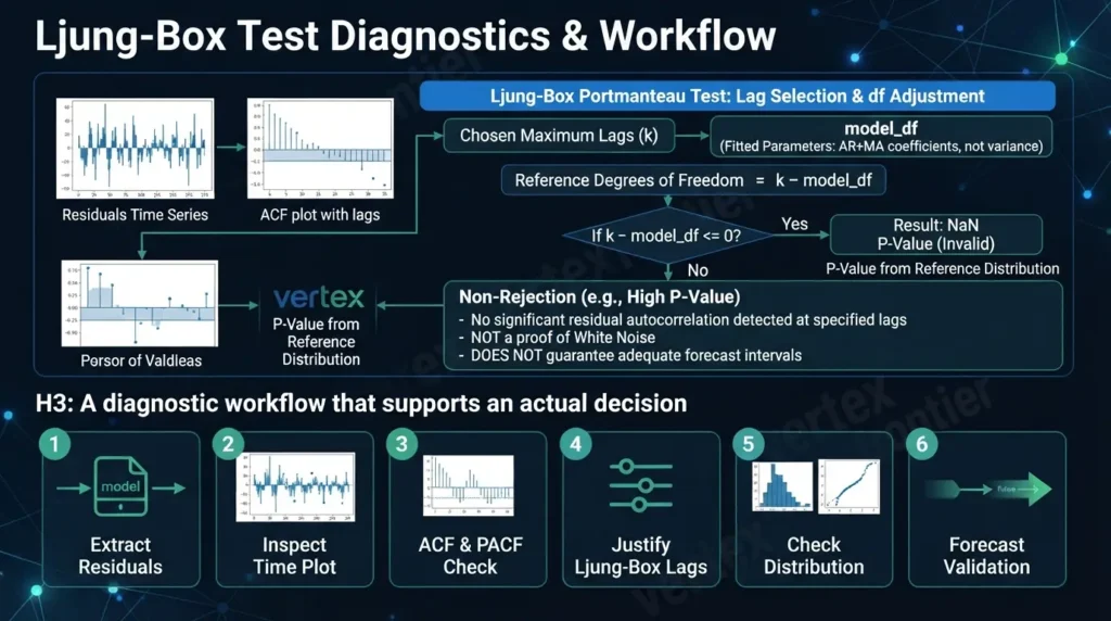
A diagnostic workflow that supports an actual decision
- Extract the appropriate innovation residuals. Check initialization effects and the package’s treatment of early observations.
- Inspect the time plot. Look for bias, outliers, changing variance, and clusters of large errors.
- Inspect ACF and, where useful, PACF. Include lags relevant to the operational horizon and seasonal cycle.
- Report a small, justified set of Ljung-Box lags. State the adjustment and ensure positive reference degrees of freedom. Do not search for a lag that yields the preferred answer.
- Check distribution and interval behavior. Long tails or changing variance can damage interval coverage without a simple residual-mean problem.
- Return to forecasting validation. A model can have clean innovation diagnostics and still forecast poorly because future X is wrong or the relationship changes.
The forecast checkresiduals reference documents its plotting and lag-selection behavior. Inspect those defaults rather than assuming every diagnostic function reports the same lag and adjustment.
A non-rejection means the test did not detect the specified dependence at those lags under its assumptions. It does not prove white noise, adequate intervals, or a production-ready forecast. Conversely, isolated ACF spikes and a joint portmanteau test answer different questions; occasional disagreement is not automatically a software bug.
Report the residual series, tested lags, adjustment rationale, and forecast evidence together.
Forecast validation: Oracle vs Available X
An ARIMAX backtest is only operationally meaningful if it recreates the information available when each forecast would have been issued. A chronological train/test split is necessary, but it does not prevent leakage from future predictors or revised historical data.
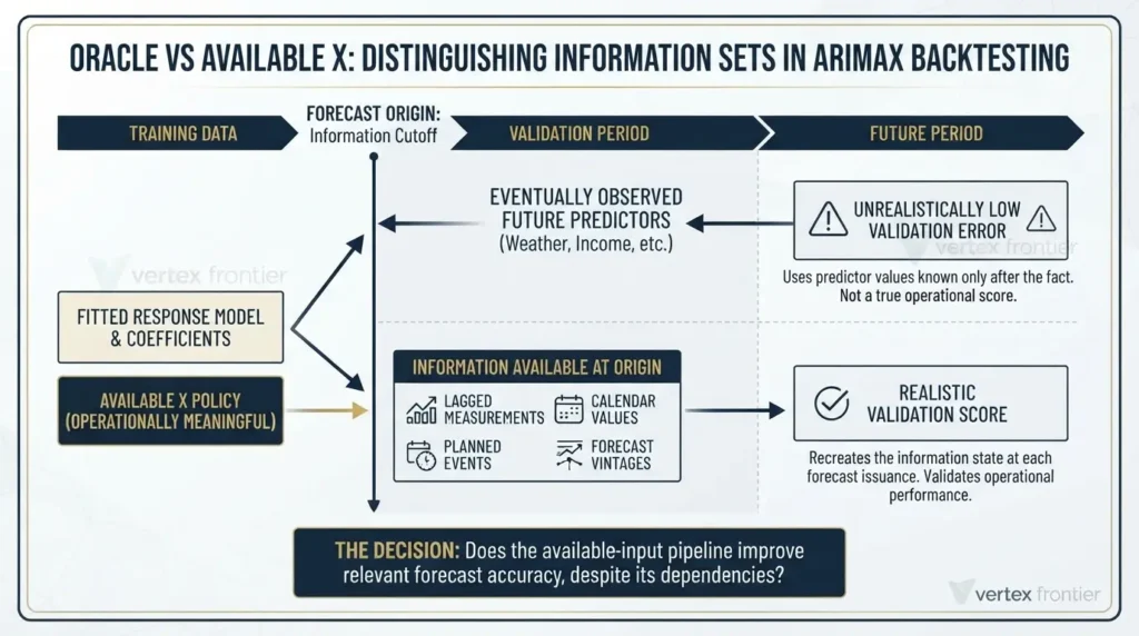
Use the Oracle vs Available X comparison to expose this distinction. Keep the fitted response model and forecast origins aligned, but evaluate two input policies:
- Oracle X: the predictor values eventually observed during the forecast period.
- Available X: calendar values, recorded plans, historical lagged measurements, forecast vintages, or assumptions that actually existed at the origin.
Oracle X is useful for studying a model conditional on correct inputs. It is not a deployment score for unknown weather, income, or other future measurements. Nor is it necessarily a numerical upper bound in every sample; forecast errors and misspecification can interact.
Warning: do not promote an oracle backtest
Click to expand or collapse warning detailsRealized future values in conditional diagnostics
If a predictor was unavailable at the forecast origin, its realized future value belongs to a conditional diagnostic experiment—not the operational validation score.
Calendar inputs and nowcasts
A genuinely known calendar input is different. A nowcast using already observed same-period X is also a different task. Label the information set before comparing results.
Step by step: rolling-origin validation
- Select historical forecast origins and a fixed horizon. Match the issuance schedule and lead times used by the business.
- Reconstruct each origin’s data snapshot. Include publication delays, revisions, planned-event versions, and the target observations available then.
- Fit preprocessing and models using that snapshot only. Predictor screening, lag selection, scaling, harmonic selection, and order tuning belong inside the training process.
- Build the future design matrix through the Covariate Contract. Refit any upstream predictor model using only its own available history.
- Forecast the full horizon without observing future Y. Updating the model after each actual arrives is valid only if that matches the intended operational task.
- Compare the baseline ladder. Include naive or seasonal-naive, univariate ARIMA/SARIMA, regression with ARIMA errors, and a transfer candidate only when justified.
- Score point and interval forecasts. Examine MAE or RMSE by lead time, interval coverage and width, and errors during events or changing regimes.
Keep the final evaluation period separate from iterative feature decisions. If many models are tried, repeatedly selecting the lowest validation error can overfit that validation set too.
Overlapping forecast horizons also produce related errors. Do not treat every forecast cell as an independent observation when making claims about uncertainty in model comparisons.
When historical predictor forecasts or plan vintages are unavailable, say so. A sensitivity analysis with degraded or delayed X can test fragility, but it is not a faithful reconstruction of past real-time forecasting.
The decision is whether the available-input pipeline improves the relevant forecast enough to justify its dependencies, not whether the regression explains more historical variance.
Forecast intervals when X is itself uncertain
OTexts explicitly notes that dynamic-regression prediction intervals omit uncertainty in forecast predictor values. A narrow interval after adding X can therefore reflect conditioning on an assumed input path, not a reduction in every source of operational uncertainty.
Distinguish three outputs:
- Known-X interval: conditional on calendar values or another genuinely supplied future path, with uncertainty from the fitted response model.
- Plug-in interval: conditional on point forecasts of unknown X. Upstream predictor uncertainty is not automatically included.
- Scenario forecast and interval: conditional on a deliberately chosen X path. It answers “under this assumption,” not “this assumption will occur.”
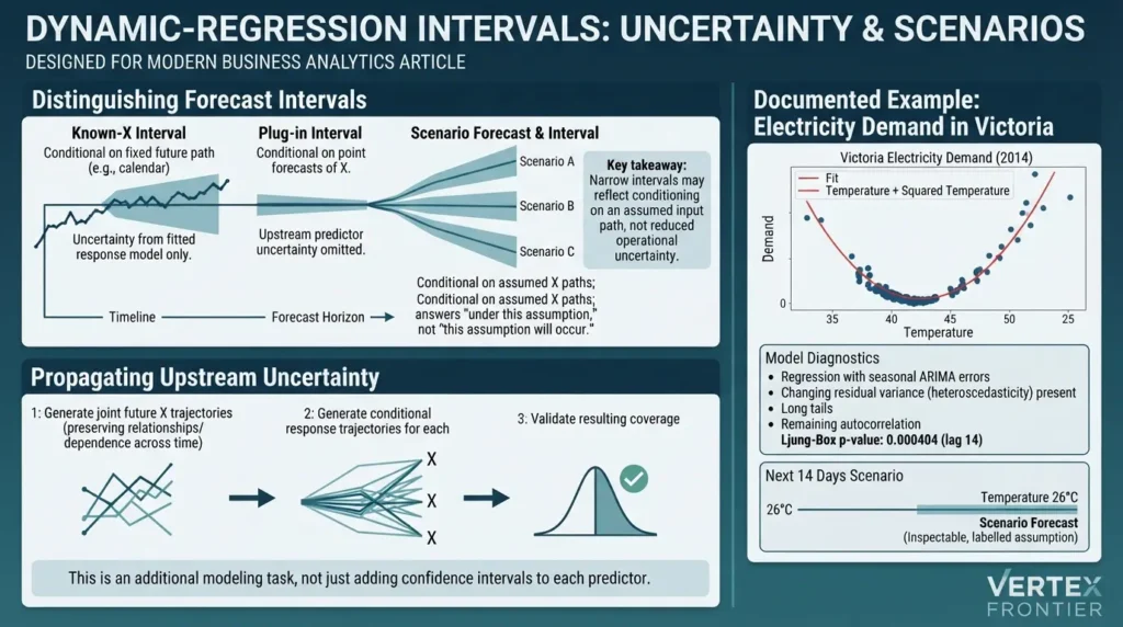
To propagate upstream uncertainty, a defensible approach is to generate joint future X trajectories, then generate conditional response trajectories for each. Preserve relationships among predictors and their dependence across time. Otherwise, simulated paths may describe combinations that the upstream process would not produce.
This is an additional modeling task, not something achieved by attaching a confidence interval to each predictor and inserting its endpoints separately. Check the treatment of parameter uncertainty as well. Validate the resulting coverage rather than assuming that added simulation makes intervals correct.
If you lack a credible probabilistic model for X, present transparent scenarios. Do not assign scenario probabilities without a defensible basis.
Documented example: electricity demand in Victoria
The FPP3 electricity-demand example uses daily data for Victoria, Australia, in 2014. Demand varies with temperature and day type, and the displayed relationship is U-shaped: heating and cooling can both increase demand.
The textbook uses temperature, squared temperature, and a working-day indicator in a regression with seasonal ARIMA errors. This shows that “linear regression” means linear in coefficients; it does not forbid a curved relationship represented by transformed predictors.
The fitted example still has diagnostic problems. The source reports changing residual variance, long tails, and remaining autocorrelation. Its published Ljung-Box calculation at lag 14, using six AR/MA coefficients as the adjustment, gives a p-value of 0.000404. That is the textbook’s reported diagnostic convention and result, not a universal seasonal adjustment or a new test performed here.
For the next 14 days, the example sets temperature to a constant 26 degrees and uses known calendar information. That is explicitly a scenario, not a claim that the weather bureau predicted exactly that path.
The outcome is an inspectable scenario forecast with documented limitations, not a measured operational accuracy improvement. The transferable lesson is to model the response shape, retain residual diagnostics, and label the future-input assumption.
Common ARIMAX mistakes and their fixes
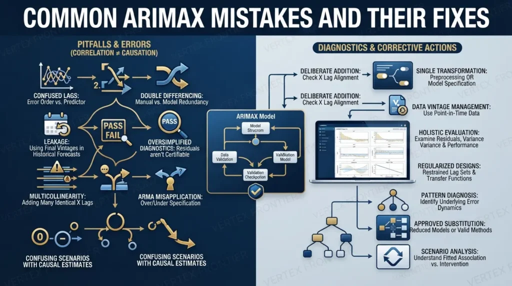
Mistaking an error order for predictor lags
ARIMA orders govern the error process in regression-with-errors models. Add delayed X columns deliberately, with availability and alignment checks.
Manually differencing twice
Check whether differencing happens in preprocessing or inside the fitted model. Keep one explicit transformation specification.
Using final data vintages in historical forecasts
Revised statistics and finalized business plans can contain later information. Preserve snapshots or disclose that real-time reconstruction is unavailable.
Treating residual diagnostics as a pass/fail certificate
State the residual type, lags, and model_df or fitdf. Examine variance, event errors, and forecast performance too.
Adding many nearly identical X lags
Adjacent lags can be highly correlated, making individual coefficients unstable. Compare restrained lag sets, a structured transfer response, or other regularized designs instead of treating every CCF spike as a required feature.
Assuming extra ARMA terms are always the cure, or always wrong
Remaining dependence may reflect error dynamics, missing calendar structure, a delayed input, a break, or data problems. Diagnose the pattern before choosing the remedy.
Silently filling missing future X with zero
Zero is a substantive input value unless your encoding defines otherwise. Use an approved substitution or a separately fitted reduced model.
Calling a scenario a causal estimate
A forecast under a changed price or promotion input relies on the fitted association continuing to hold. It does not establish what an intervention would cause.
When not to use ARIMAX
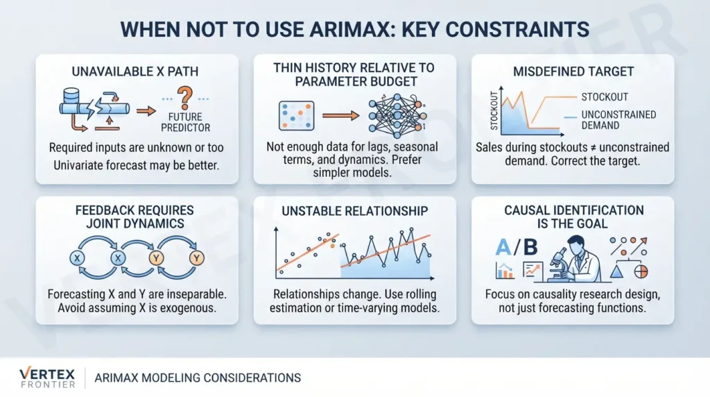
ARIMAX is not an automatic upgrade. Avoid it, or change the modeling design, when one of these constraints dominates:
- The required X path is unavailable or too uncertain. A univariate forecast may be more useful than a model that depends on inputs nobody can supply.
- History is thin relative to the parameter budget. Predictor lags, seasonal terms, transfer parameters, and error dynamics all consume information. Simpler or pooled models deserve a comparison.
- The target is misdefined. Sales during a stockout are not the same as unconstrained demand. Correct the forecasting target or use a design that addresses the observation process.
- Feedback requires joint dynamics. If forecasting X is inseparable from forecasting Y, treating X as externally given may be an awkward model of the task.
- The relationship is unstable. Compare rolling estimation, interventions, or time-varying models rather than assuming one fixed slope remains valid.
- The real objective is causal identification. Start with an appropriate research design, not a forecasting function.
Feature-rich nonlinear problems may also favor supervised lag-feature models. Many related short series may benefit from pooling. Those alternatives need the same available-X discipline; changing the model family does not remove forecasting-information constraints.
Community reports are mixed. An r/datascience demand-forecasting discussion describes stockouts, promotions, unclear demand definitions, and planner review. Treat that as community experience, not proof that SARIMAX universally fails or another algorithm universally wins.
A useful contrarian option is to keep a difficult predictor outside the mean forecast and use it as a monitoring or review signal. That can be preferable when it provides warning information but has no reliable future trajectory. It is an operational choice, not a statistical guarantee.
A production checklist for the complete forecast
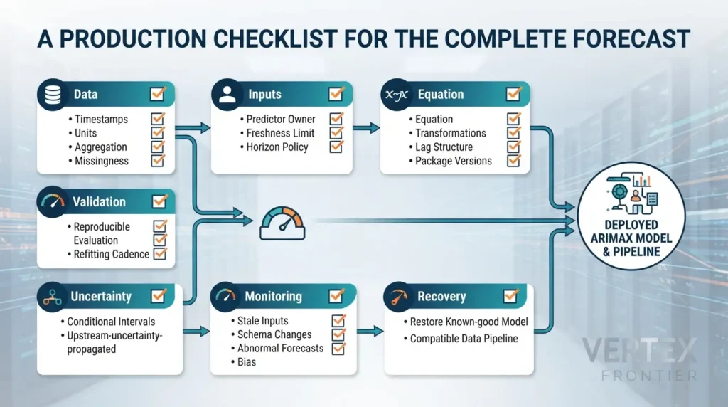
A deployed ARIMAX model is a model plus its input supply chain. Before release, confirm that you can answer these questions:
- Data: are timestamps, units, aggregation, missingness, censoring, and revisions explicit?
- Inputs: does each predictor have an owner, freshness limit, horizon policy, and approved fallback?
- Model: are the equation, transformations, lag structure, package versions, and fit status recorded?
- Validation: does the evaluation reproduce available X, refitting cadence, and the full forecast horizon?
- Uncertainty: are intervals labeled conditional, plug-in, scenario, or upstream-uncertainty-propagated?
- Monitoring: can you detect stale inputs, schema changes, abnormal forecasts, bias, and deteriorating coverage?
- Recovery: can you restore a known-good model with its compatible data and feature pipeline?
- Lineage: can you distinguish forecasts issued at different origins for the same target date?
In an r/datascience thread on putting forecasts into production, commenters recommend versioned artifacts, retained inputs, rollback, and experiments with retraining cadence. These are practitioner recommendations, not package requirements. Test cadence historically instead of assuming that more frequent retraining is always better.
For many series, batch scoring and stored artifacts may be sufficient; a permanently running endpoint is not an inherent ARIMAX requirement. Keep architecture proportional to the decision’s latency needs.
For the broader learning sequence, the Data Science collection connects stationarity checks and ARIMA fundamentals. In production, the same sequence should be backed by reproducible data snapshots and forecast records.
Conclusion
Integrate explanatory variables only after defining how they enter the equation and how their future values will be supplied. Then validate that complete process, not a better-informed version built with hindsight.
The Covariate Contract keeps feature selection tied to reality. Prewhitening narrows lag hypotheses. Model-aware diagnostics check the remaining dependence. Available-X validation decides whether the extra information earns its operational cost. If that case is weak, keeping the simpler baseline is a sound forecasting decision.
Frequently asked questions
What is the difference between ARIMA, ARIMAX, and SARIMAX?
ARIMA models a response using its own temporal dynamics. ARIMAX adds external regressors, although the name does not uniquely specify their mathematical treatment. SARIMAX commonly adds seasonal ARIMA errors and regressors; the Statsmodels class can also fit non-seasonal models. State the equation and software options before interpreting results.
Can SARIMAX forecast without future exogenous values?
A fitted model that uses exogenous inputs needs the future design values required for its forecast horizon. Supply known values, lagged observations where available, separately forecast inputs, or explicit scenarios. If none is defensible, shorten the horizon or fit a model without that dependency. Past coefficients do not eliminate the need for future inputs.
How do I fit ARIMAX in R: Arima or TSA::arimax?
Use forecast::Arima with a numeric xreg matrix for regression with ARIMA errors, and supply a compatible future matrix when forecasting. TSA::arimax also offers transfer-filtered xtransf covariates. Choose it when that structure is required, and verify its transfer conventions and initialization in the pinned release. The similar names do not make the functions interchangeable.
Do exogenous variables always need to be differenced?
No. Specify a stationary relationship or model a defensible long-run relationship explicitly. A levels regression with integrated errors has an equivalent transformed representation, and some software performs that transformation internally. An already stationary input does not require manual differencing merely because Y is integrated. Avoid accidental double differencing and state the coefficient’s scale.
How many lags of X should I include?
Start with plausible timing and the forecasting horizon. Prewhitened CCF patterns can suggest a small candidate set, but they do not uniquely determine the model. Compare explicit lags or transfer responses using diagnostics and rolling-origin validation. Confirm the library’s CCF sign convention and whether each lagged value will actually be available.
Can an ARIMAX coefficient be interpreted as a causal effect?
Not from the forecasting specification alone. The coefficient is a conditional regression association on the modeled scale. Feedback, common shocks, selection, and omitted variables can undermine causal interpretation. A transfer response describes modeled dynamics but also needs a separate identification argument before being called causal.
Why can Ljung-Box fail to reject when the residual ACF has spikes?
The ACF examines individual lags, while Ljung-Box summarizes dependence through a chosen maximum lag. Results also depend on sample size, initialization, variance behavior, and the degrees-of-freedom convention. Verify the innovation residuals, selected lags, and model_df or fitdf. Non-rejection is not proof of white noise or a useful forecast.

Was this article helpful?