
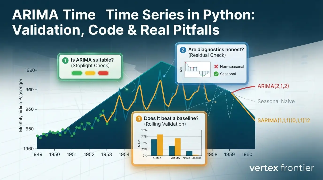

I took a common non-seasonal ARIMA recipe and ran it on a classic forecasting dataset: monthly airline passengers from 1949 to 1960. The model looked fine on a standard residual check. Then I gave the same data to a baseline that takes one line of code, and the ARIMA model lost on the 12-month holdout.
That result is the point of this guide. In this experiment the model did not fail because ARIMA mathematics is weak. It failed because the workflow around it was weak: nobody checked whether the data suited a non-seasonal model, whether the diagnostic was measuring what it appeared to measure, or whether the model beat something trivial.
Most tutorials teach you to fit the model. This one teaches you to choose it, test it, trust it, and walk away from it when needed. You will get a three-gate framework, working Python code, and an experiment you can reproduce yourself, with the data source, software versions and raw results listed.
Evaluation Gates
Click any topic to expand or collapseGate 1: Is ARIMA suitable?
A Stoplight check that sorts your data into Green, Yellow or Red before you write any code.
Gate 2: Are diagnostics honest?
A statsmodels gotcha that makes a failing model look perfect, and the one-line fix.
Gate 3: Does it beat a baseline?
Rolling-origin validation against naive benchmarks, with real numbers from the airline dataset.
Evidence, not folklore
What the M5 competition, a flu-forecasting study and a benchmark paper actually found.
What ARIMA Actually Does
ARIMA (Autoregressive Integrated Moving Average) is a statistical model that forecasts a single time series from its own past values and past forecast errors, after removing trend through differencing.
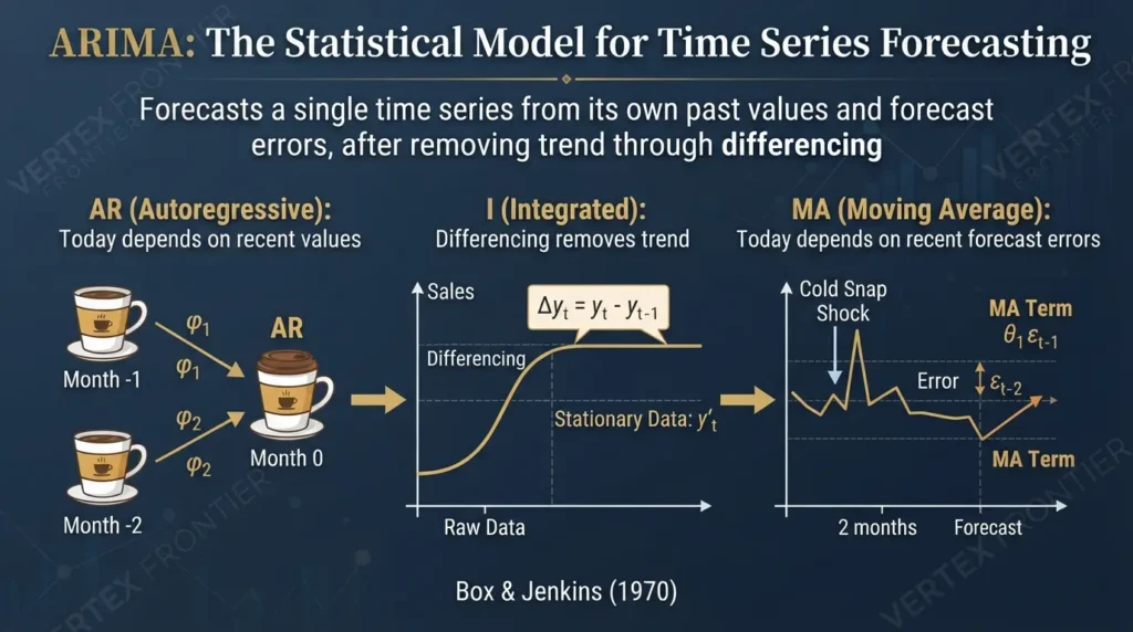
It answers one narrow question: does this series have memory, and can that memory be modeled? Box and Jenkins formalized the approach in 1970, and it is still taught and used today. The model has three parts.
- AR (autoregressive): today’s value depends on recent values.
- I (integrated): the series is differenced to remove trend.
- MA (moving average): today’s value depends on recent forecast errors.
Picture monthly sales for a coffee brand. Last month’s sales pull this month’s number (AR). A cold snap two months ago caused a surprise spike, and the model learns to correct for that kind of shock (MA). Sales also grow year over year, so you difference the series first to get a stable signal (I).
Notice the MA part has nothing to do with the moving average on a stock chart. It models how past mistakes echo into the present.
The AR Component in One Formula
Here is the AR(p) model. The parameter p says how many past values the model looks at.
AR(p) MODEL
yt = c + φ1yt−1 + φ2yt−2 + … + φpyt−p + εt
c is a constant, each φ is a weight on a past value, ε is random noise.
A φ near 0.9 means yesterday carries strongly into today. A φ near 0.2 means the series forgets quickly. Try it below with an AR(1) model.
Enter a constant, a persistence weight (φ) and the previous value to see the expected next value.
ARIMA combines momentum (AR), shock correction (MA) and trend removal (I). It is simple in concept, and the difficulty lies in the workflow.
Gate 1: The ARIMA Readiness Test
Before opening a notebook, ask whether this series is a candidate at all. Five questions settle most cases.
- Is it one variable? ARIMA models a single series. If promotions, weather or policy drive your numbers, you probably want ARIMAX, which adds external regressors.
- Is the pattern mostly linear? Heavy non-linearity and explosive volatility break the model.
- Is the spacing regular? Irregular timestamps need preprocessing.
- Is the horizon short to medium? Forecasts flatten as the horizon grows. More on that below.
- Are there structural breaks? A merger, a regulation or a pandemic splits your data into two different processes.
The statsmodels ARIMA class handles seasonal terms and exogenous regressors in the same interface, so upgrading is cheap. See the statsmodels ARIMA documentation for seasonal_order and exog.
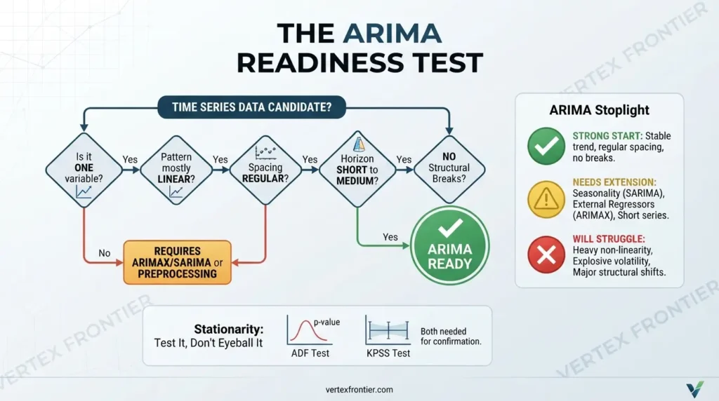
The ARIMA Stoplight
Use this editorial framework to sort your situation in two minutes. It is a heuristic assembled from the sources in this guide, not an empirically validated rule, so treat the thresholds as starting points.
- Stable or removable trend
- Short to medium horizon
- No seasonality, or it has been handled
- No structural break in the modeling window
- Roughly 100 or more clean, regular observations
- Clear seasonality: use SARIMA
- Known external drivers: use ARIMAX
- Mild structural break: add an intervention dummy
- Short series: select models with AICc
- Strong non-linearity or explosive volatility
- Several overlapping seasonalities
- Intermittent demand with many zeros
- Very long horizons
- Major structural shifts inside the window
Stationarity: Test It, Don’t Eyeball It
A stationary series has a constant mean, stable variance and consistent autocorrelation over time, with no trend and no growing swings.
Two tests are standard, and they ask opposite questions.
- ADF test: the null hypothesis is a unit root, meaning non-stationary. A small p-value rejects it. The statsmodels adfuller documentation explains the options and notes that in version 0.15.0 the function still returns a plain tuple by default and warns about a future change, which is why the code below passes
result_object=True. The original method comes from Dickey and Fuller’s 1979 paper. - KPSS test: the null hypothesis is stationarity, either around a constant or around a trend, as the statsmodels kpssdocumentation describes. If ADF and KPSS agree, you can trust the verdict. If they disagree, investigate before modeling. We cover this in our practical guide to the KPSS test in Python.
How Much Data Do You Need?
Nobody can give you a universal number. A common practitioner rule of thumb is about 50 observations as a floor, 100 or more for comfort, and several full cycles if seasonality is present. Treat it as a heuristic, not a law.
What is well established is the small-sample correction: Hurvich and Tsai’s paper on regression and time series model selection in small samples derives a bias-corrected AIC (AICc) for that situation, and it penalizes complexity more when data is scarce.
Choosing p, d and q Without Guesswork
Most people obsess over p and q. Get d right first, because everything else depends on it.
How to choose d, step by step:
- Plot the series and look for trend or growing variance.
- If variance grows, apply a log or Box-Cox transformation first.
- Run ADF (and KPSS) on the series.
- If it is non-stationary, difference once and test again.
- Rarely go beyond d = 2 (a practitioner rule of thumb). If you seem to need more, suspect a structural break or non-linearity.
A common workflow is to transform first, then difference. This is my recommendation rather than a documented rule: a log transform stabilizes variance, and differencing the logged series then removes trend. The SciPy boxcox documentation covers the lambda parameter, where a value of zero corresponds to a log transform. Box-Cox also requires strictly positive data; in my test SciPy 1.17.1 raised ValueError: Data must be positive. for zeros and negative values.
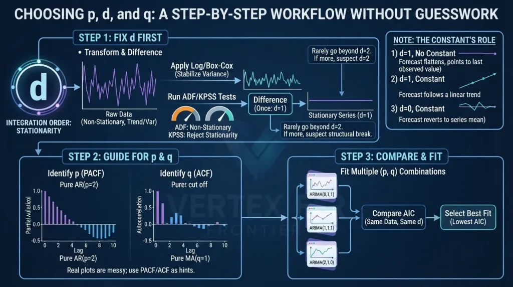
For p and q, the classic pattern guide is: PACF cuts off after lag p for a pure AR process, and ACF cuts off after lag q for a pure MA process. Penn State’s STAT 510 lesson on identifying ARIMA models shows how these patterns guide a first guess. Real plots are messy. In practice, fit several small (p, q) combinations and compare them, but only under the rule you will meet in the AIC section: same data, same differencing.
One more point most guides skip: what the constant does. Rob Hyndman’s note on constants in ARIMA models lists the long-run behavior. With d = 1 and no constant, forecasts head to a non-zero constant set by the last few observations. With d = 1 and a constant, they follow a straight line whose slope is the mean of the differenced data. With d = 0 and a constant, they go to the series mean.
For seasonal models the same rules apply with d replaced by d + D. This is why ARIMA forecasts flatten, and it matters in Python: the statsmodels ARIMA documentation says the default is a constant for models without integration and no trend for models with integration. In my test, a non-seasonal ARIMA(1,1,1) fitted to the 132 training observations of the airline data gave a flat 60-step forecast by default, while trend='t' produced a rising line.
Fix d first, transform before differencing, and treat ACF/PACF as hints rather than answers.
The Box-Jenkins Workflow
The Box-Jenkins method follows four iterative stages:
- Identification: plot, test stationarity, transform, difference, inspect ACF and PACF.
- Estimation: fit candidate models by maximum likelihood.
- Diagnostic checking: examine residuals for leftover structure.
- Forecasting: produce point forecasts and prediction intervals.
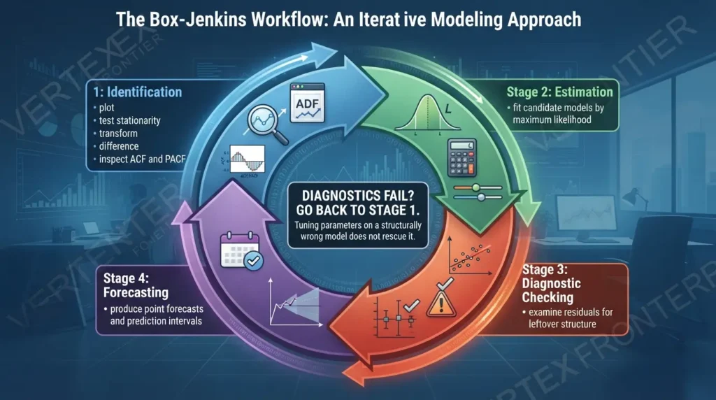
Stage 3 is the one people rush, and it is where this guide’s biggest lesson lives. If diagnostics fail, go back to Stage 1. Tuning parameters on a structurally wrong model does not rescue it.
A Worked Example: Where the Standard Recipe Breaks
Let’s use the classic airline passengers dataset: 144 monthly values from January 1949 to December 1960. It has strong trend, growing seasonal swings and a clear annual cycle. I ran everything below on October 16, 2026, holding out the final 12 months. The table lists every condition so you can reproduce the result or challenge it.
| Item | Setting |
|---|---|
| Data | 144 monthly observations, January 1949 to December 1960, from the airline-passengers.csv file in Jason Brownlee’s Datasets repository (a community copy, downloaded October 16, 2026) |
| Software | Python 3.12.3, statsmodels 0.15.0, SciPy 1.17.1, pandas 3.0.2, NumPy 2.4.4 |
| Split | Train: January 1949 to December 1959 (132 observations). Test: 1960 (12 observations) |
| Transformation | Box-Cox, lambda estimated on training data only (0.129) |
| Models | ARIMA(2,1,2) as a typical non-seasonal specification, and SARIMA(1,1,1)(0,1,1)12 with one regular difference, one seasonal difference and one seasonal MA term. Both use the statsmodels ARIMA class with default settings. The orders were not found by an exhaustive search. |
| Baselines | Naive (repeat the last value) and seasonal naive (repeat the same month of the previous year) |
| Metric | MAPE on the original scale |
| Rolling protocol | Expanding window, first origin after 84 observations, origin moves 6 months at a time, 12-month horizon, 9 windows, lambda re-estimated in every window |
If you are choosing tools for this kind of work, our guide to choosing Python data libraries covers where statsmodels fits next to pandas and others. If your data loading feels slow, see why pandas can be slow and how to fix it.
Step 1: Load, Split and Test Stationarity
Python: Load, split, test stationarity:
import numpy as np import pandas as pd from statsmodels.tsa.stattools import adfuller, kpss
df = pd.read_csv("airline.csv", parse_dates=["Month"], index_col="Month") df.index.freq = "MS" y = df["Passengers"] y_train, y_test = y.iloc[:-12], y.iloc[-12:] # 132 training months, 12 test months
adf = adfuller(y_train, result_object=True) kp = kpss(y_train, regression="c", nlags="auto", result_object=True) print("Training observations:", len(y_train)) print("ADF p-value:", round(adf.pvalue, 4)) print("KPSS p-value:", kp.pvalue)Result: the ADF p-value is 0.9929, so a unit root cannot be rejected. The KPSS p-value is 0.01, which is a boundary value: the statsmodels kpss documentation says the p-value is interpolated from a table and a boundary point is returned when the statistic falls outside it, and statsmodels prints an InterpolationWarning to say so. Read it as “p is at most 0.01”. Both tests agree that the raw series is not stationary.
Step 2: Stabilize Variance, Then Difference
Python: Box-Cox on training data, then test the differenced series:
from scipy.stats import boxcox
bc_values, lam = boxcox(y_train) bc = pd.Series(bc_values, index=y_train.index) print("Box-Cox lambda:", round(lam, 3)) print("ADF after 1 difference :", round(adfuller(bc.diff().dropna(), result_object=True).pvalue, 4)) print("ADF after 1 + seasonal (12) :", round(adfuller(bc.diff().diff(12).dropna(), result_object=True).pvalue, 4))
Lambda comes out at 0.129. After one ordinary difference, the ADF p-value is 0.0255, so the test passes at the 5% level. After adding a seasonal difference at lag 12 it is 0.0012.
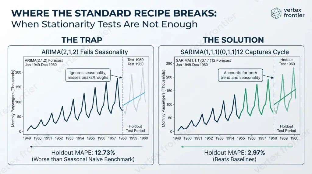
Notice what this does and does not tell you. A pass after one difference would let you proceed with a plain ARIMA. But ADF asks only about a unit root; it cannot tell you whether a non-seasonal model is adequate. In my interpretation, that is exactly the trap in this example: the stationarity test is satisfied while a seasonal pattern remains that a non-seasonal model cannot absorb.
Step 3: Inspect ACF and PACF
Python: ACF and PACF of the stationary series:
import matplotlib.pyplot as plt from statsmodels.graphics.tsaplots import plot_acf, plot_pacf
stationary = bc.diff().diff(12).dropna() fig, ax = plt.subplots(1, 2, figsize=(12, 4)) plot_acf(stationary, lags=24, ax=ax[0]) plot_pacf(stationary, lags=24, ax=ax[1]) plt.tight_layout() plt.show()
Step 4: Fit Two Models and Compare Them Against Baselines
Here is the part tutorials skip. We fit the non-seasonal ARIMA(2,1,2), a seasonal model, and two baselines that need no fitting at all.
Python: Fit ARIMA and SARIMA, forecast 12 months, compare with baselines:
from statsmodels.tsa.arima.model import ARIMA from scipy.special import inv_boxcox
def mape(actual, forecast): return float(np.mean(np.abs((actual - forecast) / actual)) * 100)
arima = ARIMA(bc, order=(2, 1, 2)).fit() sarima = ARIMA(bc, order=(1, 1, 1), seasonal_order=(0, 1, 1, 12)).fit()
forecasts = { "ARIMA(2,1,2)": inv_boxcox(arima.forecast(12), lam).values, "Naive (last value)": np.repeat(y_train.iloc[-1], 12), "Seasonal naive": y_train.iloc[-12:].values, # same month last year "SARIMA(1,1,1)(0,1,1,12)": inv_boxcox(sarima.forecast(12), lam).values, } for name, f in forecasts.items(): print(f"{name:26s} MAPE: {mape(y_test.values, f):.2f}%")
MAPE is the mean absolute percentage error: the average size of the miss as a percentage of the actual value, lower is better. It is fine here because every actual value is far from zero. FPP3’s discussion of accuracy measures explains why percentage errors break down near zero and recommends scaled errors such as MASE when you compare across series.
| Model | Holdout MAPE | Reading |
|---|---|---|
| Naive (last value) | 14.25% | Ignores seasonality |
| ARIMA(2,1,2) | 12.73% | Worse than seasonal naive |
| Seasonal naive | 9.99% | The bar to beat |
| SARIMA(1,1,1)(0,1,1)12 | 2.97% | Beats both baselines on this holdout |
Read that table twice. On this holdout, the non-seasonal ARIMA(2,1,2) was worse than repeating last year’s numbers, and the seasonal version cut the error by roughly three quarters. This is also the logic behind the baseline gate. FPP3 states the principle plainly: forecasting methods you develop should be compared with simple benchmarks, and a method that does not beat them is not worth considering.
Before vs. after:
- Before: a plausible-looking ARIMA with a tidy forecast line, no baseline, and one number nobody questioned.
- After: a baseline gate that exposes the weak specification, and a seasonal specification that earns its place.
Here is the output you should see if you run Steps 1 to 6 on the same data and versions (the InterpolationWarning from KPSS appears on stderr):
Expected output (stdout):
Training observations: 132 ADF p-value: 0.9929 KPSS p-value: 0.01 Box-Cox lambda: 0.129 ADF after 1 difference : 0.0255 ADF after 1 + seasonal (12) : 0.0012 ARIMA(2,1,2) MAPE: 12.73% Naive (last value) MAPE: 14.25% Seasonal naive MAPE: 9.99% SARIMA(1,1,1)(0,1,1,12) MAPE: 2.97% loglikelihood_burn ARIMA: 1 SARIMA: 13 First ARIMA residual: 6.494 | first training value: 6.494 ARIMA Ljung-Box p, all residuals : 0.9996 ARIMA Ljung-Box p, burn-in removed : 4.7467168640214974e-35 SARIMA Ljung-Box p, all residuals : 0.25 SARIMA Ljung-Box p, burn-in removed : 0.3941 windows: 9 mean MAPE ARIMA: 11.95 | SARIMA: 4.38 | seasonal naive: 9.42 SARIMA beats seasonal naive in 8 of 9 windows ARIMA beats seasonal naive in 2 of 9 windowsGate 2: The Diagnostic That Lies
Here is the finding I did not expect. Run the residual check on the ARIMA(2,1,2) model in two ways and compare.
Python: Residual diagnostics, naive vs. honest:
from statsmodels.stats.diagnostic import acorr_ljungbox
def ljung_box_p(fit, n_arma_params, trim=True): resid = fit.resid.iloc[fit.loglikelihood_burn:] if trim else fit.resid lags = min(24, len(resid) // 5) # 2 x period for monthly data, capped at a fifth of the sample return float(acorr_ljungbox(resid, lags=[lags], model_df=n_arma_params).iloc[0, 1])
print("loglikelihood_burn ARIMA:", arima.loglikelihood_burn, " SARIMA:", sarima.loglikelihood_burn) print("First ARIMA residual:", round(arima.resid.iloc[0], 3), "| first training value:", round(bc.iloc[0], 3)) print("ARIMA Ljung-Box p, all residuals :", round(ljung_box_p(arima, 4, trim=False), 4)) print("ARIMA Ljung-Box p, burn-in removed :", ljung_box_p(arima, 4)) print("SARIMA Ljung-Box p, all residuals :", round(ljung_box_p(sarima, 3, trim=False), 4)) print("SARIMA Ljung-Box p, burn-in removed :", round(ljung_box_p(sarima, 3), 4)) sarima.plot_diagnostics(figsize=(12, 7)) plt.tight_layout() plt.show()
On my run the numbers were:
- ARIMA(2,1,2), all residuals: Ljung-Box p-value of 0.9996. A perfect pass.
- ARIMA(2,1,2), burn-in removed: p-value of about 5 × 10⁻³⁵. A decisive fail.
- SARIMA, all residuals: p-value of 0.25. SARIMA, burn-in removed: 0.3941. Both pass, so this trap mattered mostly for the non-seasonal model.
What happened? With differencing, the first residual is not an ordinary forecast error. In my run it was 6.494, identical to the first Box-Cox value in the training series, and loglikelihood_burn was 1 for the ARIMA model and 13 for the seasonal one (the regular difference plus the seasonal difference at lag 12).
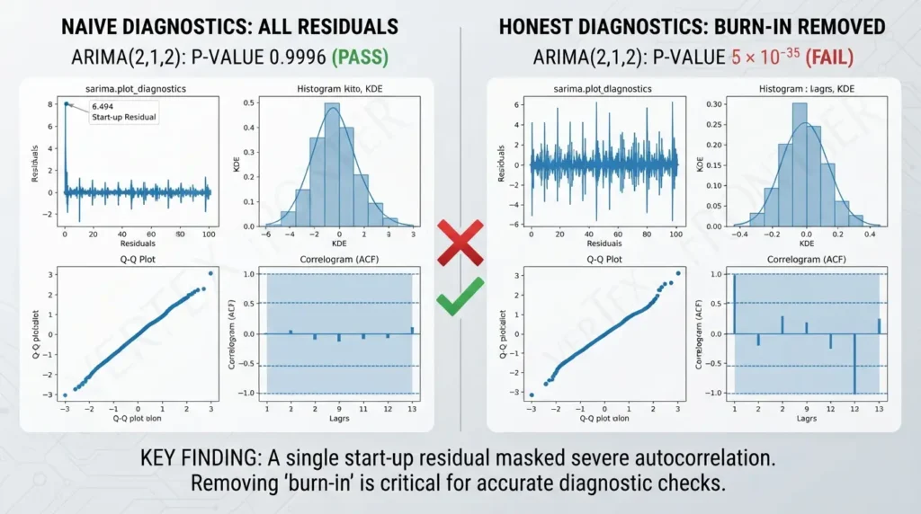
My interpretation is that these are start-up residuals, and that one huge artificial value hides the autocorrelation in the rest. I verified the behavior in statsmodels 0.15.0 by inspection, but I did not find loglikelihood_burn described in the documentation pages I opened, so treat it as observed behavior and re-check it after upgrading.
Two more details in that code come from FPP3’s section on residual diagnostics. The suggested number of lags is 10 for non-seasonal data and twice the seasonal period for seasonal data, capped at a fifth of the sample, and for ARIMA models the degrees of freedom should be adjusted. That is what model_df does in the acorr_ljungbox function. The same section adds a caution that matters here: checking residuals is important, but it is not a good way to select a forecasting method.
Rule to remember: after differencing, remove the burn-in residuals, adjust the degrees of freedom, and never treat a clean residual check as proof of forecast quality.
When Things Go Wrong: Failure Modes I Hit or Verified
| Symptom | Likely cause | What to do |
|---|---|---|
| Ljung-Box passes, forecast loses to a baseline | Start-up residuals included, or a non-seasonal model on seasonal data | Remove loglikelihood_burn residuals and compare with seasonal naive |
ConvergenceWarning after fitting a high-order model | Over-parameterized model; observed for ARIMA(3,1,3) on this data | Lower the order, and do not trust that fit’s AIC |
ValueError: Data must be positive. | Box-Cox applied to zeros or negative values | Use a different transformation, or shift the data only with a documented reason |
FutureWarning from adfuller or kpss | The plain-tuple return is being phased out; the default is due to change in a later release | Pass result_object=True and read .pvalue, as in the code above |
| Long-horizon forecast is a flat line | d = 1 with no constant, which is the statsmodels default for integrated models | Consider a shorter horizon; add trend='t' only if steady drift is justified |
| KPSS p-value is exactly 0.01 or 0.1 | Statistic is outside the lookup table, so a boundary value is returned | Read it as “at most 0.01” or “at least 0.1” |
ValueWarning about frequency information | Index has no frequency set; statsmodels inferred monthly start in my test | Set df.index.freq explicitly, and fix irregular dates before modeling |
The AIC Trap
AIC (Akaike Information Criterion) scores a model by rewarding fit and penalizing the number of parameters. Lower is better, but only among comparable models.
INFORMATION CRITERIA
AIC = 2k − 2 ln(L)
AICc = AIC + 2k(k + 1) / (n − k − 1)
k = number of parameters, L = maximized likelihood, n = number of observations
There are two traps here, and the second is the one almost nobody mentions.
- Trap 1: AIC measures in-sample fit. It cannot tell you how a model behaves on a different time period. Use it to shortlist candidates, then validate out of sample. The small-sample correction (AICc) comes from Hurvich and Tsai’s work on model selection in small samples.
- Trap 2: AIC is invalid across different differencing orders. Hyndman and Athanasopoulos note that comparing information criteria is only valid for ARIMA models with the same orders of differencing. The reason is that differencing changes the data the likelihood is computed on.
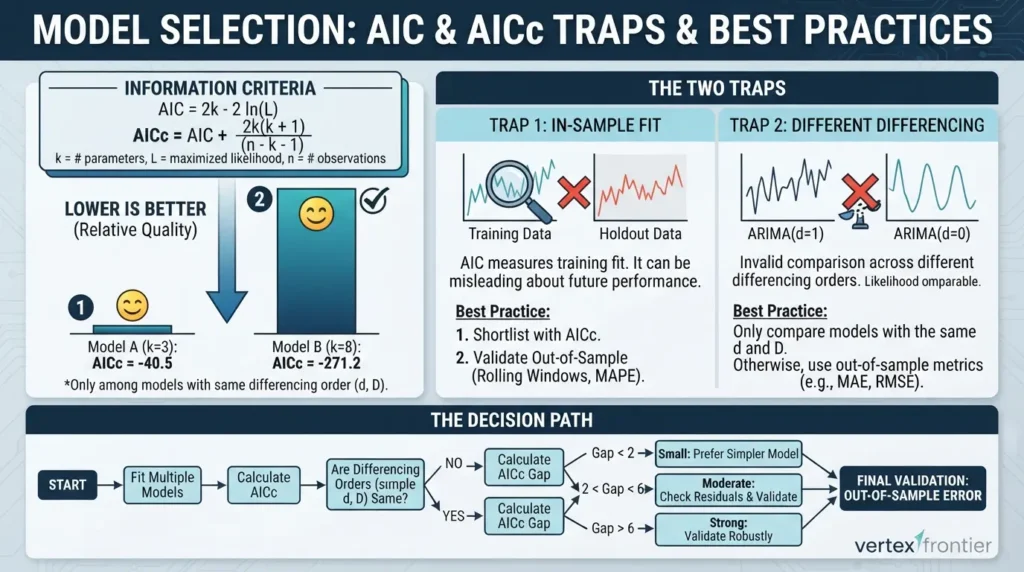
My experiment makes the danger concrete. The ARIMA(2,1,2) model had an AIC of −40.5 and the seasonal model had −271.2 (AICc −40.0 and −270.9). The gap looks enormous, and the seasonal model is indeed better on the holdout, but the two numbers are not on the same scale because the differencing differs. The verdict came from out-of-sample error, not from the AIC gap.
A small grid search shows the first trap. Among 16 non-seasonal candidates (p and q from 0 to 3, d = 1), ARIMA(3,1,3) had the lowest AIC at −66.9, but its fit raised a ConvergenceWarning, and its holdout MAPE was 8.48%, still behind the seasonal model. Its burn-in-removed residuals failed the Ljung-Box test as well. The next best candidates, ARIMA(3,1,2) at −44.5 and ARIMA(2,1,1) at −43.3, fit without warnings. A low AIC from a fit that did not converge is not a result.
Use the calculator below. It computes AIC and AICc from the formulas above and refuses to give a verdict when the differencing differs. Its default input values are illustrative placeholders, not results from the experiment.
Enter log-likelihood and parameter count for two models fitted on the same data.
The thresholds in the calculator (2 and 6) are common rules of thumb rather than hard laws. Treat them as prompts to look closer.
AIC shortlists. Out-of-sample validation decides.
Gate 3: Rolling-Origin Validation Against a Baseline
One train/test split tells you how a model did in one window. Time series change, so you want to know how it does across many.
How rolling-origin validation works, step by step:
- Train on the first T observations.
- Forecast the next h steps and record the error.
- Move the origin forward and retrain on a longer history.
- Repeat until you run out of data.
- Look at the whole error distribution, not just the mean.
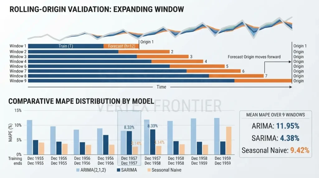
FPP3’s section on time series cross-validation calls this evaluation on a rolling forecasting origin, notes that the earliest observations are not used as test sets, and describes how to adapt it to multi-step errors. It is also the habit that separated serious M5 entrants: according to the competition paper, the top four methods and most of the top 50 validated on at least the last four 28-day windows.
Python: Rolling-origin validation (expanding window):
def rolling_mape(order, seasonal=(0, 0, 0, 0), start=84, horizon=12, step=6): scores = [] for t in range(start, len(y) - horizon + 1, step): b, l = boxcox(y.iloc[:t]) # lambda from the training window only fit = ARIMA(pd.Series(b, index=y.index[:t]), order=order, seasonal_order=seasonal).fit() pred = inv_boxcox(fit.forecast(horizon), l) scores.append(mape(y.iloc[t:t + horizon].values, pred)) return scores
def rolling_seasonal_naive(start=84, horizon=12, step=6): return [mape(y.iloc[t:t + horizon].values, y.iloc[t - 12:t].values) for t in range(start, len(y) - horizon + 1, step)]
a = rolling_mape((2, 1, 2)) s = rolling_mape((1, 1, 1), (0, 1, 1, 12)) n = rolling_seasonal_naive() print("windows:", len(a)) print("mean MAPE ARIMA:", round(np.mean(a), 2), "| SARIMA:", round(np.mean(s), 2), "| seasonal naive:", round(np.mean(n), 2)) print("SARIMA beats seasonal naive in", sum(x < z for x, z in zip(s, n)), "of", len(s), "windows") print("ARIMA beats seasonal naive in", sum(x < z for x, z in zip(a, n)), "of", len(a), "windows")| Training ends | ARIMA(2,1,2) | SARIMA | Seasonal naive |
|---|---|---|---|
| Dec 1955 | 13.61% | 1.69% | 13.49% |
| Jun 1956 | 10.53% | 3.68% | 10.92% |
| Dec 1956 | 13.63% | 1.83% | 10.76% |
| Jun 1957 | 10.46% | 6.68% | 7.34% |
| Dec 1957 | 10.88% | 8.33% | 3.14% |
| Jun 1958 | 11.59% | 2.68% | 6.25% |
| Dec 1958 | 13.97% | 7.59% | 11.06% |
| Jun 1959 | 10.16% | 3.96% | 11.83% |
| Dec 1959 (the holdout) | 12.73% | 2.97% | 9.99% |
| Mean of 9 windows | 11.95% | 4.38% | 9.42% |
Three things stand out.
- The seasonal model beat the seasonal naive baseline in 8 of 9 windows, and the non-seasonal ARIMA beat it in only 2 of 9.
- The seasonal model is not uniformly safe. In the window ending December 1957, seasonal naive scored 3.14% and the SARIMA model 8.33%. A single split could have hidden that.
- Single-window errors for the seasonal model ranged from 1.69% to 8.33%. The 2.97% on the final holdout is below the 4.38% average, so reporting only that number would have promised more than the model reliably delivers.
The windows overlap and share most of their training data, so they are not independent trials. They show spread, not statistical proof.
A model earns trust by beating a baseline across many windows and by showing where it does not.
Prediction Intervals: Tell People How Wrong You Might Be
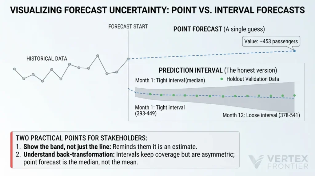
A point forecast is a single guess. A prediction interval is the honest version, and FPP3 goes as far as saying point forecasts can be of almost no value without it.
For the seasonal model, the 95% interval for the first forecast month ran from about 393 to 449 passengers around a central value of 420. By month 12 it widened to roughly 378 to 541 around 453. The model is telling you that near-term numbers are tight and far-term numbers are loose.
Two practical points.
- Show the band, not just the line: Stakeholders remember a line forever. A band reminds them it is an estimate. Eleven of the 12 holdout values fell inside their intervals here, but 12 points cannot establish that the intervals are well calibrated.
- Know what back-transformation does: FPP3 explains that intervals computed on a transformed scale and then back-transformed keep their coverage but are no longer symmetric, and that the simple back-transformed point forecast is usually the median of the forecast distribution rather than the mean. The difference matters when you add forecasts together. See FPP3’s section on forecasting with transformations.
- It covers one series, so it says nothing general about ARIMA or SARIMA accuracy.
- ARIMA(2,1,2) was not tuned, and SARIMA orders were not searched, so neither is the best its family can do.
- It uses one error metric, a 12-observation holdout and nine overlapping windows.
- It does not compare ETS, Prophet or machine learning models.
- Behavior such as
loglikelihood_burnand the default trend belongs to statsmodels 0.15.0 and may change. Exact decimals can vary across versions and optimizers.
Outliers: Four Types, Four Different Problems
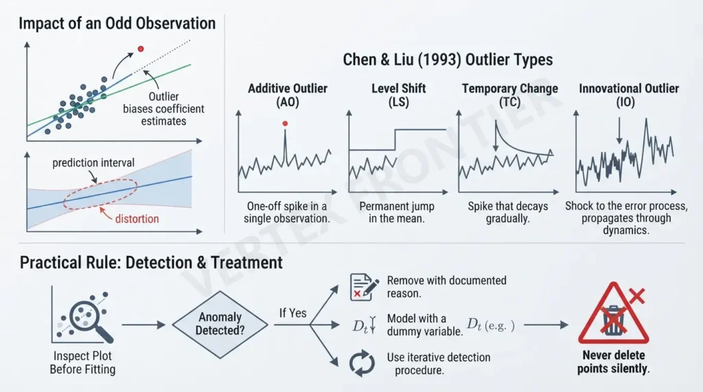
A single odd observation can bias coefficient estimates and distort prediction intervals. That is general statistical practice, not a result from this guide’s experiment. Chen and Liu’s 1993 paper on joint estimation of model parameters and outlier effects describes four types.
- Additive outlier (AO): a one-off spike in a single observation.
- Level shift (LS): a permanent jump in the mean, such as a regulation change.
- Temporary change (TC): a spike that decays gradually, like a promotion that fades.
- Innovational outlier (IO): a shock to the underlying error process that propagates through the model dynamics.
A separate 1993 study by Chen and Liu on forecasting with outliers, summarized in an IAOR abstract, reports, citing earlier work, that forecast intervals are quite sensitive to additive outliers while point forecasts are largely unaffected unless the outlier is near the forecast origin.
Practical rule: inspect the plot before fitting. Then either remove the anomaly with a documented reason, model it with a dummy variable, or use an iterative detection procedure. Never delete points silently.
What Real Evidence Says About ARIMA
Theory is cheap. Here is what documented studies found, including where ARIMA lost. Each case separates what the authors report from my interpretation.
Case Study 1: One ARIMAX Beat the Ensembles in Flu Forecasting
Challenge: produce short-term forecasts of influenza hospitalizations for 48 US states across the 2022 to 2024 seasons, using National Healthcare Safety Network data.
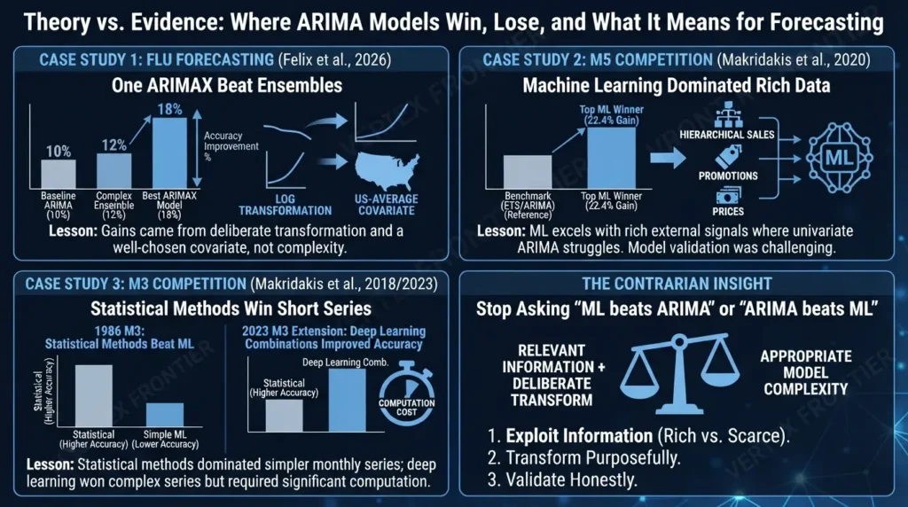
Action: in a 2026 study in the Journal of the Royal Society Interface, Felix, Rohani and Drake compared 29 approaches. They included ARIMA and ARIMAX models with different covariates, ensembles of two sizes, and variants that forecast on a log scale and back-transform. The reference points were an automatically tuned ARIMA without a log transform and the FluSight baseline, scored with weighted interval scores.
Outcome: according to the authors’ abstract, the log-and-back-transform approach improved performance the most, the average of hospitalizations across the contiguous US was the most useful covariate, ensembles typically did not improve performance, and the best model was an automatically tuned ARIMAX with that covariate and the log-back transformation. The abstract reports no accuracy figures, so I quote none; check the full paper before citing numbers.
Lesson (my interpretation): the gains came from a transformation and one well-chosen covariate, not from stacking more models. That echoes this guide’s workflow: transform deliberately, and add information before adding complexity.
Case Study 2: The M5 Competition, Where ARIMA’s Family Lost
This one is a failure story, and it is more instructive than a success. Figures below come from the authors’ October 2020 preprint of the M5 Accuracy competition paper; the published version is in the International Journal of Forecasting, 2022.
Challenge: forecast 42,840 hierarchical daily sales series from Walmart, 28 days ahead. The data came with prices, calendar events and promotion indicators, and many series were intermittent, meaning they contained many zeros. The competition drew 5,507 teams.
Action: the organizers published 24 benchmarks, including exponential smoothing and ARIMA variants, and used the best of them, a bottom-up exponential smoothing method, as the reference.
Outcome: all of the top 50 submissions were machine learning methods, all beat that benchmark by more than 14%, and the winner beat it by 22.4%. Yet only 415 teams (7.5%) beat the benchmark with the forecasts they selected. The paper adds that 672 teams (12.2%) would have beaten it had they chosen their own best submission, which it attributes probably to misleading validation scores. At the most granular product-store level, the average gain of the top methods over the benchmark was only about 3%.
Where ARIMA fits: within the benchmark set, the paper reports that an ARIMA variant with explanatory variables was 13% more accurate than the same family without them.
Lesson: the data was rich, cross-correlated and full of external signals, which is where univariate ARIMA has the least to offer. My reading is that it sits in the Red column of the Stoplight. The second lesson is about validation: many teams could not tell which of their own submissions was best.
Case Study 3: When Machine Learning Lost Instead
A 2018 PLOS ONE study by Makridakis, Spiliotis and Assimakopoulos compared popular machine learning methods against eight statistical methods on 1,045 monthly series from the M3 competition. The authors report that the ML methods were dominated across all accuracy measures and forecasting horizons, and that they needed more computation.
The picture has moved since. A 2023 study in the Journal of the Operational Research Society by the same group, which extended the M3 comparison to deep learning models, reports that combinations of deep learning models performed better than most standard statistical and machine learning models, especially for monthly series and long-term forecasts, at the cost of significantly increased computational time.
The Contrarian Insight
Here is the claim that survives all three cases, and it is my reading rather than a finding of any one study: “ML beats ARIMA” and “ARIMA beats ML” are both the wrong question.
M5 shows ML winning when there is rich information to exploit. The M3 study shows statistical methods winning on short monthly series. The flu study shows a modest model winning because it was given a transformation and a useful covariate. What the cases share is that the winners used relevant information, and the M5 paper shows that validating honestly was hard even for experienced teams.
Seven Common ARIMA Mistakes (and Fixes)
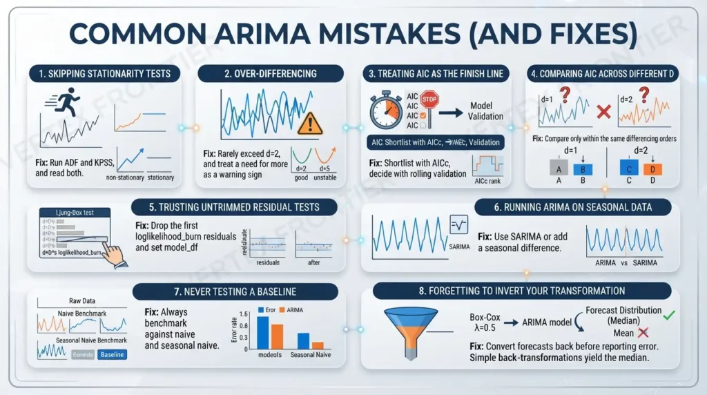
Skipping stationarity tests
Fix: run ADF and KPSS, and read both.
Over-differencing
Fix: rarely exceed d = 2, and treat a need for more as a warning sign.
Treating AIC as the finish line
Fix: shortlist with AICc, decide with rolling validation.
Comparing AIC across different d
Fix: compare only within the same differencing orders.
Trusting untrimmed residual tests
Fix: drop the first loglikelihood_burn residuals (here, d plus D times s) and set model_df when running Ljung-Box.
Running ARIMA on seasonal data
Fix: use SARIMA or add a seasonal difference.
Never testing a baseline
Fix: always benchmark against naive and seasonal naive.
There is a related mistake worth naming: forgetting to invert your transformation. If you fit on Box-Cox data, forecasts must be converted back before you report any error. Note that the simple back-transformed forecast is usually the median of the forecast distribution rather than the mean, according to FPP3’s section on forecasting with transformations, which matters if you add forecasts together.
The Forecast Trust Ladder
Before deploying, a model should clear five rungs. The thresholds below are for you to fix before you look at the results, because a pass condition chosen afterward is not a test.
| Rung | Test | Pass condition to define in advance | A pass does not prove |
|---|---|---|---|
| 1. Fit | Fit the final specification and inspect warnings | No convergence warnings; coefficients are plausible | That the model forecasts well |
| 2. Residuals | Ljung-Box with burn-in removed, model_df set, lags per FPP3 | p-value above the threshold you chose, plus no pattern in the residual plots | That it is better than a simple method |
| 3. Baseline | Rolling-origin error against naive and seasonal naive | Beats both in at least the share of windows you fixed in advance | That future windows will behave the same way |
| 4. Plausibility | Domain review of forecast and interval | A domain owner can explain the forecast through known drivers | That unknown drivers are absent |
| 5. Monitoring | A plan for drift and retraining | A retraining schedule, a tracked error metric and an alert threshold exist before launch | That the alert will fire early enough |
H2: When to Stop Tuning and Switch
Decision matrix: if you see this, consider that. Each row names the evidence, and most of it comes from the cases above, so the scope is narrower than the advice may sound.
| Signal | Consider | Evidence and scope |
|---|---|---|
| A persistent seasonal pattern; seasonal naive beats your non-seasonal ARIMA | A seasonal specification (seasonal_order) | Airline example: 12.73% to 2.97% holdout MAPE. One series. |
| Residuals track an external variable you will know over the forecast horizon | ARIMAX (exog) | M5 benchmark: ARIMA variant with explanatory variables about 13% more accurate. Flu study: best model was an ARIMAX. Different domains. |
| Strong seasonality and you want automatic model selection | ETS as an alternative | Per FPP2, ARIMA is not simply more general than ETS; each includes models the other lacks. |
| Many related series, rich covariates, lots of data | Global machine learning models | All top 50 M5 entries were ML. Retail sales; do not generalize beyond similar data. |
| Many zeros (intermittent demand) | Intermittent-demand methods such as Croston’s | In the M5 paper, Croston’s method beat seasonal naive at the three most granular levels, by roughly 13% to 27%. |
| Residuals stay non-linear after every ARIMA variant | Hybrid or ML approaches | My inference from the cases above, not a tested threshold. |
| Nothing you try beats seasonal naive in rolling windows | Stop tuning; use the baseline, or get more data | FPP3: a method that does not beat simple benchmarks is not worth considering. |
Conclusion
ARIMA has outlasted decades of newer models because, used with discipline, it is honest. It states its assumptions, and it tells you when they fail, if you let it.
The discipline comes down to three gates. Check suitability before you code. Make sure your diagnostics are measuring what you think they are. Prove the model beats a baseline across many windows, not one. The airline experiment shows what happens when you skip them: a model that passes a flawed check and loses to a one-line baseline.
Reproduce the code, change the orders, and break it on purpose. That habit teaches more than any formula.
FAQ
What is ARIMA used for?
ARIMA forecasts a single time series from its own past values and past forecast errors, after differencing to remove trend. It is typically used for short-horizon forecasting of one regularly spaced series. A documented example is a 2026 study in the Journal of the Royal Society Interface, where an ARIMA model with an exogenous variable gave the best forecasts of influenza hospitalizations among 29 approaches compared.
How do I choose p, d and q?
Choose d first: test stationarity and difference until the series passes, rarely going beyond two differences. Then use ACF and PACF plots to suggest candidate values of p and q, compare a small set of candidates with AICc only among models that share the same differencing, and confirm the choice with honest residual checks and rolling-origin validation against simple baselines.
When should I use SARIMA instead of ARIMA?
Use a seasonal specification when the data repeats on a fixed cycle, such as monthly data with a yearly pattern, or when a seasonal naive baseline beats your non-seasonal model. In the airline passengers example in this guide, adding one seasonal difference and a seasonal moving-average term cut the 12-month holdout error from 12.73% to 2.97% MAPE. That is one dataset, so run the same comparison on your own series.
Should I transform before or after differencing?
A common workflow is to transform first, for example with a log or Box-Cox transformation to stabilize variance, and then difference to remove trend. Box-Cox requires strictly positive data. After forecasting, convert the results back to the original scale; the simple back-transformed forecast is usually the median of the forecast distribution rather than the mean.
Why does my ARIMA forecast flatten out?
Long-run ARIMA forecasts depend on the differencing order and the constant. With one difference and no constant, forecasts head toward a constant value; with one difference and a constant, they follow a straight line. In statsmodels 0.15.0 the ARIMA class includes no trend by default when the model is integrated, so a model with d equal to 1 levels off unless you pass trend=’t’. Add a trend only if a steady drift is justified for your series.
Why did my model pass the Ljung-Box test but forecast badly?
Two separate things can go wrong. First, with differencing the first residuals are start-up values, not real forecast errors; in statsmodels you can drop the first loglikelihood_burn residuals before testing, and in the airline example doing so changed the ARIMA p-value from 0.9996 to effectively zero. Second, a residual check is not a way to choose a forecasting method, so also confirm that the model beats naive and seasonal naive baselines in rolling-origin validation.
Can I compare AIC across ARIMA models with different differencing?
No. Information criteria are only comparable between ARIMA models with the same orders of differencing, because differencing changes the data on which the likelihood is computed. To compare models that differ in d or D, such as a non-seasonal and a seasonal model, use out-of-sample error from a holdout or rolling-origin validation.
Is ARIMA still relevant in 2026?
It depends on the problem. A 2026 influenza-hospitalization study found a single ARIMAX model outperformed ensembles of autoregressive models, while in the M5 retail competition all of the top 50 submissions were machine learning methods that beat every statistical benchmark, including ARIMA variants. ARIMA-family models remain useful as interpretable baselines and for single series that you can validate honestly, but they are not the best choice for every forecasting problem.

Was this article helpful?




[…] stationarity is confirmed, the next decision is the forecasting model itself, our complete guide to ARIMA walks through when it works, when it fails, and why a baseline can beat […]
[…] same logic extends to time series: fitting an ARIMA model lives in Statsmodels, not scikit-learn, precisely because the value is in the residual diagnostics, […]