
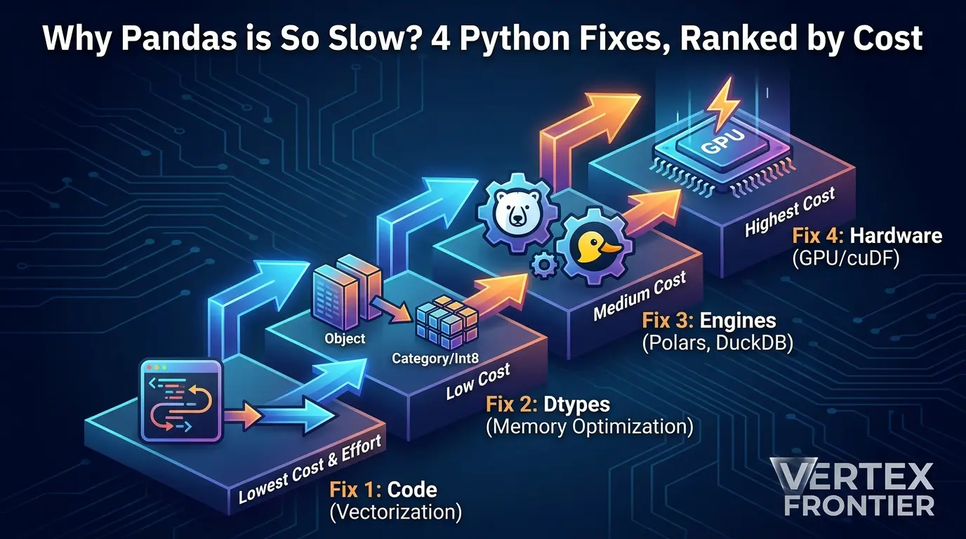

Search for why pandas is so slow and most answers tell you to leave. Install Polars. Try DuckDB. Rent a GPU. Buy a faster laptop.
We tested that advice against something less exciting: the code you already wrote. One ordinary analytics job, written four ways over the same 200,000 rows on pandas 3.0.6, took 5.7 seconds with an iterrows loop and 0.03 seconds with whole-column operations. No new library was involved.
That result changes the order in which you should try things. If your code loops over rows, a faster engine is a faster interpreter for a problem that was never about interpreter speed.
This article rebuilds that argument and puts it under stress. We check each claim against the pandas documentation, NVIDIA’s published results, independent benchmarks, and a spot-check we ran ourselves. Where a number did not hold up, we say so instead of printing it.
Here is what you will get:
- A 90-second method to find out which of four bottlenecks you actually have
- Four fixes, ordered from cheapest to most expensive, with the evidence for each
- Honest ranges instead of single headline multipliers
- A pandas 3.0 twist that quietly changes old memory advice
- Two calculators and a decision tool you can use on your own numbers
Quick takeaways
Click any point to expand or collapseProfile first
Read call counts, not seconds. It takes about 90 seconds.
Fix 1, your code
Replace row loops with whole-column operations. Our spot-check: roughly 190x.
Fix 2, your dtypes
Category plus downcasting cuts memory and speeds up compute as a side effect.
Fix 3, the engine
Polars and DuckDB win mostly when they read the file themselves.
Fix 4, hardware
cuDF can run pandas code on a GPU, but the numbers come from NVIDIA, not independent tests.
How to Read the Numbers in This Article
Benchmark numbers travel badly. A headline like “300x faster” hides the workload, the row count, the hardware and the library version. So every figure below carries one of three labels:
- Spot-check: our own test on pandas 3.0.6, Polars 2.0.0 and DuckDB 1.5.6 (Python 3.12), run in a single-core Linux sandbox at 200,000 to 3 million rows. Absolute seconds depend on hardware, so read the ratios.
- NVIDIA-published: vendor results, attributed as such and never stated as universal facts.
- Docs: statements taken from official documentation.
The workload is simple and realistic. Compute revenue and a channel fee for each order, keep only completed orders, then group by region and channel. Every variant was checked against the others before any timing was recorded, so a fast but wrong answer fails instead of winning a chart. That habit alone is worth copying. The data is synthetic and randomly generated.
One more note. Engines move quickly, and Polars now ships in a 2.x line. Treat the engine ratios as a snapshot, not a ranking.
What Does “Pandas Is Slow” Actually Mean?
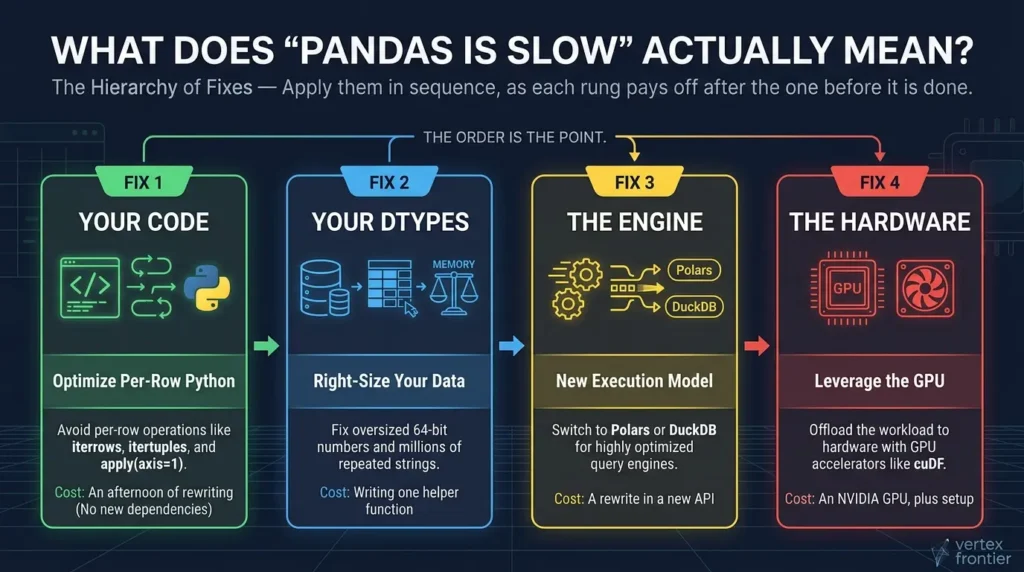
Pandas feels slow when your job spends its time in one of four places: your own per-row Python code, oversized data types, the execution engine underneath, or the CPU itself. Each place has its own fix, and each fix has a very different price.
Per-row Python: iterrows, itertuples, apply(axis=1).
Cost: an afternoon of rewriting. No new dependency.
64-bit numbers holding tiny values. Millions of repeated strings.
Cost: one helper function.
Polars or DuckDB doing the same work with a different execution model.
Cost: a rewrite in a new API.
Moving the job to a GPU with cuDF.
Cost: an NVIDIA GPU, plus setup.
The order is the point. Each rung only pays off after the one above it is done. Move to a faster engine while your code still loops row by row and you have bought a faster interpreter for a problem that wasn’t about interpreter speed.
When the loop is pure Python rather than pandas, the deeper question is usually whether the nesting itself is pointing at a design flaw, our guide to nested loops in Python walks through the diagnostic before you reach for a faster engine.
Here is the part most guides skip: the swap everyone talks about is often the smallest win on the table. In our spot-check, Polars beat tuned in-memory pandas by 1.8x and DuckDB was 2.4x slower. Rewriting the loop was worth roughly 190x. codecut.ai’s CSV-reading test reported 7.7x for Polars but only 1.4x for DuckDB on the same task, which shows how much these ratios depend on what you run.
Diagnose first. Then pick the cheapest fix whose symptoms match yours.
Step 0: Profile with cProfile Before Fixing Anything
Why does this step come first? Because three of the four fixes are wasted if you apply them to the wrong problem.

How to find your pandas bottleneck in 90 seconds:
- Wrap the slow job in a single function.
- Run it under cProfile on a realistic sample of your data.
- Sort by call count, not by time.
- Match the top entries to one of the four signatures below.
Python Code: profile by call count:
import cProfile import pstats profiler = cProfile.Profile() profiler.enable() revenue_by_region(df) # your slow function profiler.disable() stats = pstats.Stats(profiler) stats.sort_stats("ncalls").print_stats(10) # Memory check for the dtype question: print(df.memory_usage(deep=True).sum() / 1e6, "MB")Why call counts? Profiling slows the code it watches. In our spot-check, the same 20,000-row loop took 2.23 seconds under cProfile against 0.68 seconds plain, about 3.3x longer, so wall time inside a profile is inflated. Call counts are the stable signal. Even then, treat them as approximate rather than exact. The Python profiler documentation covers cProfile and pstats.
What a Loop-Bound Profile Looks Like
Take the classic slow version: a for loop over df.iterrows() with four column reads, one multiplication and one dictionary lookup per row. Profiling a 2,000-row run on pandas 3.0.6 gave these call counts:
- About 352,000 function calls in total, roughly 176 per row.
- Series.__getitem__ ran exactly 8,000 times, 4 per row, once per column read.
- isinstance ran about 101,000 times, roughly 50 type checks per row.
- A new Series object was built for every row the loop yielded.
Now look at what is missing. Nothing in that top ten is arithmetic. The multiplication you asked for is too cheap to make the list. That is the diagnosis. The mechanism matches the pandas documentation for iterrows, which explains that every row comes back as a Series and that dtypes are not preserved across rows. The same page recommends itertuples as a generally faster alternative that preserves dtypes.
Expert insight: A flat profile, with time spread across real compute such as group-by, merge and sort, means your code is not the problem. That is when the engine question becomes worth asking. A profile flooded with Series.__getitem__ and isinstance means no engine can save you.
Tap the symptom that sounds like your job.
How Long Will the Full Run Take?
You profiled a sample. Now you want to know whether the full job takes ten minutes or ten hours. For a per-row loop, the projection is simple, because the cost per row stays almost flat. In our spot-check, an iterrows loop cost between 22.5 and 24.6 microseconds per row at every size from 20,000 to 400,000 rows.
That rule has a limit. It holds for row loops. It does not hold for vectorized code or for engines: in the same test, a vectorized group-by cost 0.93 microseconds per row at 20,000 rows and 0.08 at 400,000, because fixed overhead dominates small samples. Use the projection to size a loop, not to predict a fixed-up job.
Full runtime = sample runtime × (full rows ÷ sample rows)
Try 20,000 rows, 0.47 seconds and 50,000,000 rows. You get about 19.6 minutes. Half a second on the sample turns into a coffee break at full size, and a slower loop or a bigger table pushes it into hours.
Profile, read the call counts, and match the signature. It costs 90 seconds and saves the afternoon you would have spent on the wrong fix.
Fix 1: Stop the Loop with Vectorization
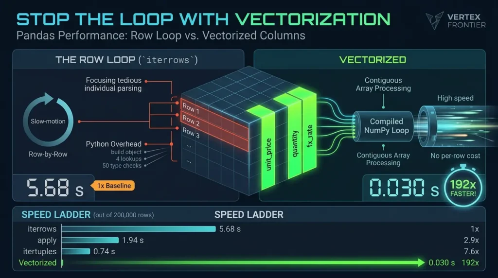
Wondering why iterrows is so slow? It pays Python interpreter overhead on every single row: build an object, do four lookups, run 50 type checks. The column version hands one contiguous buffer to one compiled loop inside NumPy, and the per-row cost disappears because nothing per row is left.
What is vectorization in pandas? Vectorization means operating on whole columns as contiguous arrays handed to compiled loops, instead of paying Python interpreter overhead once for every row. It is why df["a"] * df["b"] can beat a loop doing the same multiplication by two orders of magnitude.
The Before and After in Code
Python Code: the row loop (illustrative schema):
FEE_RATE = {"web": 0.029, "retail": 0.015, "partner": 0.040, "mobile": 0.025} def revenue_loop(df): net = [] for _, row in df.iterrows(): gross = row["unit_price"] * row["quantity"] * row["fx_rate"] net.append(gross - gross * FEE_RATE[row["channel"]]) out = df.assign(net_revenue=net) out = out[out["status"] == "completed"] return out.groupby(["region", "channel"], as_index=False)["net_revenue"].sum()Python Code: the same job, no loop:
def revenue_vectorized(df): done = df[df["status"] == "completed"] gross = done["unit_price"] * done["quantity"] * done["fx_rate"] net = gross - gross * done["channel"].map(FEE_RATE) return (done.assign(net_revenue=net) .groupby(["region", "channel"], as_index=False)["net_revenue"].sum())The column names are our illustration of a typical orders workload. The shape is what matters: multiply whole columns, map the fee rate off the channel column, subtract. Filtering first also means the arithmetic runs on fewer rows.
The Speed Ladder: How Much Does Each Rewrite Buy?
| Method | Time (200,000 rows) | Speedup versus iterrows |
|---|---|---|
| iterrows loop | 5.68 s | 1x (baseline) |
| apply(axis=1) | 1.94 s | 2.9x |
| itertuples loop | 0.74 s | 7.6x |
| Vectorized columns | 0.030 s | 192x |
Read the table with care, because the middle rows teach the most.
apply(axis=1) is not vectorization. It is still a Python function called once per row, so it bought only 2.9x in our spot-check. Marc Garcia's walkthrough gives the same rule for pandas: never make the Python interpreter run loops, whether you wrote them yourself or asked pandas to run them through DataFrame.apply.
itertuples is the real "use the faster loop" answer. It bought 7.6x in our spot-check. Faster, but still a loop.
So "stop using iterrows" is correct advice, but it is not the whole advice. Stopping the loop is the fix. Making the loop faster is a consolation prize.
How big is the vectorization win? 192x in our spot-check, at 200,000 rows on pandas 3.0.6. The multiplier moves with row count, dtypes and what the loop does per row, so quote it as "two orders of magnitude on this workload," never as a constant.
How to replace a row loop with vectorized code:
- List every column the loop reads and every value it writes.
- Rewrite each arithmetic line as an operation on whole columns.
- Replace dictionary lookups with Series.map (or a merge for bigger lookup tables).
- Replace if branches with boolean masks or numpy.where.
- Compare against the old output with pandas.testing.assert_frame_equal before you time anything.
If plain vectorization still isn't enough, the pandas user guide has dedicated pages on Enhancing performance and Scaling to large datasets.
Do the Math on Your Own Job
How much is a speedup worth? Use the formula, then the calculator.
Speedup = slow runtime ÷ fast runtime
Time saved (%) = (1 − fast runtime ÷ slow runtime) × 100
Try 5.7 and 0.03, the loop and vectorized times from our 200,000-row spot-check. You get roughly 190x.
Can Pandas Handle 10 Million Rows?
Yes. In our spot-check, the vectorized job processed 1 million rows in about 0.11 seconds on a single core. Marc Garcia's walkthrough goes much further: about 120 million flight records in 22 CSV files, roughly 13 GB on disk, on a single 16 GB laptop with pandas 1.4.4. Loading everything at once is likely to raise a MemoryError. His tuned pandas version, with only the needed columns and compact dtypes, finished in about 2 minutes 45 seconds with a peak near 8.1 GB. Reading one year at a time cut the peak to about 900 MB and the time to about 37 seconds. Case Study 2 below has the full ladder.
The practical limit is rarely row count. It is memory, and how you read the data.
Rewriting the loop is the cheapest large win in pandas. It needs no new dependency, no new API and no second copy of your data.
Fix 2: Optimize Memory with Category and Downcasting
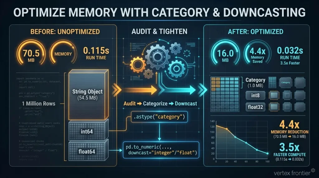
This fix is almost as cheap as the first, and far fewer people try it. In our spot-check, one helper function took a 1-million-row orders frame from 70.5 MB to 16.0 MB, and the identical vectorized code then ran about 3.5x faster as a side effect, from 0.115 seconds down to 0.032 seconds.
Audit First: Which Columns Are Worth Converting?
Don't convert blindly. This audit measures every column and tests the category conversion on the column itself, so the cardinality warning later in this section becomes a number instead of a guess.
Python Code: audit a DataFrame before converting anything:
import pandas as pd def audit_dataframe(df): rows = [] for col in df.columns: s = df[col] mb = s.memory_usage(deep=True) / 1e6 distinct = s.nunique(dropna=True) tip = "keep as is" if pd.api.types.is_string_dtype(s) or s.dtype == object: cat_mb = s.astype("category").memory_usage(deep=True) / 1e6 tip = (f"category: {mb:.1f} -> {cat_mb:.1f} MB" if cat_mb < 0.5 * mb else "leave as string (too many distinct values)") elif pd.api.types.is_integer_dtype(s): small = pd.to_numeric(s, downcast="integer").dtype if small != s.dtype: tip = f"fits {small} today (min {s.min()}, max {s.max()}); check future ranges" elif pd.api.types.is_float_dtype(s): tip = "float32 possible, but loses precision" rows.append((col, str(s.dtype), round(mb, 1), distinct, tip)) out = pd.DataFrame(rows, columns=["column", "dtype", "MB", "distinct", "suggestion"]) return out.sort_values("MB", ascending=False, ignore_index=True) print(audit_dataframe(df).to_string(index=False))Sample output: synthetic 1,000,000-row orders frame, pandas 3.0.6:
column dtype MB distinct suggestion status str 16.0 2 category: 16.0 -> 1.0 MB channel str 13.5 4 category: 13.5 -> 1.0 MB region str 9.0 4 category: 9.0 -> 1.0 MB order_id int64 8.0 1000000 fits int32 today (min 0, max 999999); check future ranges unit_price float64 8.0 1000000 float32 possible, but loses precision quantity int64 8.0 9 fits int8 today (min 1, max 9); check future ranges fx_rate float64 8.0 1000000 float32 possible, but loses precisionRead it like this. The three status-like columns shrink 9x to 16x as categories. order_id would fit a smaller integer today, but it is a unique key that will keep growing, so leave it alone. quantity fits int8 today, so confirm the real business range before you commit. The float columns trade precision, so decide column by column. The audit only recommends. You apply the changes.
Then Tighten the Columns You Chose
The helper does three things:
- Converts low-cardinality string columns to category
- Downcasts integers to the smallest type that fits
- Downcasts 64-bit floats to 32-bit (this one trades precision, see the traps below)
Python Code: a dtype-tightening helper:
import pandas as pd def tighten(df, category_cols): out = df.copy() for col in category_cols: out[col] = out[col].astype("category") for col in out.select_dtypes("integer"): out[col] = pd.to_numeric(out[col], downcast="integer") for col in out.select_dtypes("float"): out[col] = pd.to_numeric(out[col], downcast="float") return out slim = tighten(df, ["region", "channel", "status"]) print(df.memory_usage(deep=True).sum() / 1e6, "->", slim.memory_usage(deep=True).sum() / 1e6, "MB")The Pandas 3.0 Twist: PyArrow Strings by Default
Most memory advice online was written for pandas 2.x, where a string column arrives as object dtype: millions of separate Python string objects with a pointer to each.
That changed. The pandas 3.0 release notes describe a dedicated str dtype as the new default, backed by PyArrow when it is installed. A codecut.ai newsletter on the change cites about 50% lower memory. Our own spot-check on pandas 3.0.6 found a bigger gap for very short strings: one million values from a four-word vocabulary took 54.5 MB as object and 13.5 MB as str, about 4x. String length and repetition change the ratio, so measure your own columns.
One condition matters. The release notes say the new dtype falls back to NumPy object storage when PyArrow isn't installed, so without PyArrow you get the new behavior but not the memory win.
Expert insight: "Use categoricals to save memory" was advice against object. On pandas 3 with PyArrow installed, the baseline moved. Measure with memory_usage(deep=True) before assuming category will still pay off.
What Category and Downcasting Actually Save
| Stage | Memory result | Label |
|---|---|---|
| String column, 4 distinct values, 1M rows, as object | 54.5 MB | Spot-check, pandas 3.0.6 |
| Same column as the new str dtype | 13.5 MB (about 4x smaller) | Spot-check, pandas 3.0.6 |
| Same column as category | 1.0 MB (about 54x smaller than object) | Spot-check, pandas 3.0.6 |
| Numeric columns, 1M rows: int64 to int8, float64 to float32 | 16.0 MB to 5.0 MB (3.2x) | Spot-check, pandas 3.0.6 |
| Whole 7-column orders frame after the tighten helper | 70.5 MB to 16.0 MB (4.4x) | Spot-check, pandas 3.0.6 |
The first three rows are one column. The last two show what the helper does to numbers and to a whole frame. Your ratios will depend on string length and how many distinct values you have.
Why does category help so much? The official categorical guide states that a categorical's memory grows with the number of categories plus the length of the data. Store each distinct string once, then store small integer codes for the rows.
Why It Speeds Up Compute Too
On a str column, map looks up a million strings in a dictionary. On a category column, it looks up the handful of categories once and reuses the integer codes underneath. In our spot-check, map over one million channel values dropped from 0.095 seconds to 0.0007 seconds, about 140x. The whole vectorized job, run on raw dtypes and then on the tightened frame, dropped from 0.115 seconds to 0.032 seconds, about 3.5x, and the totals matched to about one part in a billion.
The mechanism is documented and measurable, but the multipliers belong to this workload, so expect yours to differ. The two fixes compound: Fix 1 removes the loop, and Fix 2 shrinks what the remaining vectorized code has to touch.
Two Dtype Traps: TypeErrors and Cardinality Gotchas
Trap 1: the categorical-multiply TypeError
map on a categorical column hands back a categorical. Multiply it and pandas raises a TypeError. We reproduced this on pandas 3.0.6: the mapped result kept the category dtype, and multiplying it failed. The categorical guide states that arithmetic operators raise TypeError on categorical data. Adding .astype("float64") to the mapped line fixed it. The exact error text varies between pandas versions, so don't paste it into a test assertion.
Python Code: the one-line fix
fee = slim["channel"].map(FEE_RATE).astype("float64") # category in, float64 out net = gross - gross * feeTrap 2: category can cost more than object:
If almost every value is unique, such as order IDs or email addresses, the categories array is as large as the data. The same docs warn that in this case a categorical can use about as much memory as an equivalent object column, or more. Convert columns with a handful of distinct values. Leave high-cardinality columns alone.
How to tighten dtypes safely:
- Measure first with memory_usage(deep=True).
- Convert only columns whose distinct values are tiny compared with the row count.
- Downcast integers and check that future values will still fit.
- Don't downcast money or other precision-sensitive floats without a reason.
- Re-run assert_frame_equal (with check_dtype=False if needed) and measure memory again.
Downcasting has two sharp edges. For floats, float32 keeps roughly seven significant digits. In our spot-check, gross revenue computed after downcasting differed from the float64 result by up to 2.1e-7 in relative terms. That is fine for a chart and wrong for a ledger. For integers, downcast picks the smallest type that fits the values present today, and arithmetic on narrow integers can wrap around silently when later data grows: in our test, an int8 value of 100 times 2 returned -56. Check ranges before you ship.
On pandas 3 you already got part of the win for free. Convert low-cardinality columns, downcast with care, and measure before and after.
Fix 3: Let an Engine Own the Read (Polars and DuckDB)
Now the fix everyone asks about. Polars is a Rust DataFrame library with a lazy query planner in front of it. DuckDB is an in-process analytical database, so your workload becomes SQL. Both return the same frame as the pandas version.
If you want the wider map of when each library fits, our guide on choosing a Python data library in 2026 compares pandas, Polars, DuckDB and Dask side by side.
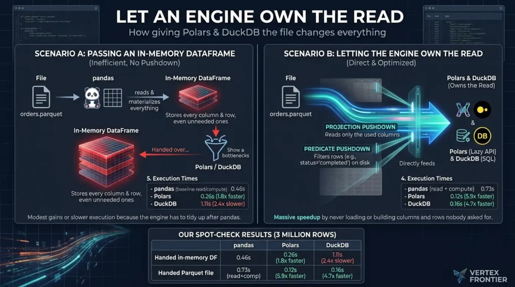
Same Engines, Two Very Different Results
Hand each engine a DataFrame that already lives in memory and the gain is modest. In our 3-million-row spot-check, Polars beat tuned pandas by 1.8x, and DuckDB was slower than the pandas code you already had.
Start from the Parquet file instead, which is what a real script usually does, and the picture changes. Both engines won clearly, 4.7x to 5.9x faster than pandas reading the same file. The table further down has the numbers.
Why? If an engine is handed a DataFrame, it is tidying up after pandas has already materialized every column. If it is handed the file, it can push the projection, the filter and the scan down into the read, and never build the columns nobody asked for.
Our Spot-Check Shows the Same Pattern
We ran the same revenue job on 3 million rows with pandas 3.0.6, Polars 2.0.0 and DuckDB 1.5.6, once handing each engine an in-memory DataFrame and once handing it the Parquet file.
| Input | pandas (vectorized) | Polars | DuckDB |
|---|---|---|---|
| Handed an in-memory DataFrame | 0.46 s | 0.26 s (1.8x faster) | 1.11 s (2.4x slower) |
| Handed the Parquet file | 0.73 s (read plus compute) | 0.12 s (5.9x faster) | 0.16 s (4.7x faster) |
DuckDB loses on a materialized DataFrame and wins when it owns the read. Details and limits: median of five runs after a warm-up run, 3 million rows, results checked for equality on a smaller sample first, and the Polars in-memory time includes converting from pandas. The sandbox had a single CPU core, so multithreaded engines could not show their full advantage. The gap may look different on your machine, which is why the benchmark protocol later in this article matters.
Expert insight: Engines don't only change speed. They change what you are bound by. A job that was memory-bound in pandas often becomes I/O-bound in an engine that skips unneeded columns and row groups.
What are projection and predicate pushdown?
Projection pushdown means reading only the columns a query uses. Predicate pushdown means applying filters during the scan so that unneeded rows are never loaded. Columnar formats such as Parquet make both cheap. If you want to see where Parquet stops and table formats begin, our piece on how Parquet files differ from table formats like Iceberg picks up exactly where this section ends.
Python Code: DuckDB reading the Parquet file directly:
import duckdb result = duckdb.sql(""" SELECT region, channel, SUM(gross - gross * CASE channel WHEN 'web' THEN 0.029 WHEN 'retail' THEN 0.015 WHEN 'partner' THEN 0.040 ELSE 0.025 END) AS net_revenue FROM (SELECT region, channel, unit_price * quantity * fx_rate AS gross FROM 'orders.parquet' WHERE status = 'completed') GROUP BY region, channel """).df()The Polars version of the same job uses its lazy API. scan_parquet doesn't load anything. It records a plan, and nothing runs until collect(). That gap is what lets Polars push the filter and the column selection into the read.
Python Code: Polars lazy query over the Parquet file:
import polars as pl FEE_RATE = {"web": 0.029, "retail": 0.015, "partner": 0.040, "mobile": 0.025} lazy = ( pl.scan_parquet("orders.parquet") .filter(pl.col("status") == "completed") .with_columns( gross=pl.col("unit_price") * pl.col("quantity") * pl.col("fx_rate"), fee_rate=pl.col("channel").replace_strict(FEE_RATE, return_dtype=pl.Float64), ) .with_columns(net_revenue=pl.col("gross") - pl.col("gross") * pl.col("fee_rate")) .group_by("region", "channel") .agg(pl.col("net_revenue").sum()) ) print(lazy.explain()) # inspect the optimized plan first result = lazy.collect() # the query runs hereWe ran this snippet on Polars 2.0.0 against a small Parquet file and checked the output by hand. It uses our illustrative schema. Two details to know:
- replace_strict raises an error if a channel is missing from FEE_RATE. That is useful here, because a silent null would quietly corrupt revenue. Pass a default= value only if you want a fallback.
- On a real file, print lazy.explain() and look at the scan step. If the plan shows the filter and only the columns you use at the scan, Polars owns the read, which is the effect described above.
Polars has also changed fast between 1.x and 2.x, so check the release notes if a method name differs in your version.
Which Tool for Which Input?
| Tool | Works best when | Switching cost | Evidence in this article |
|---|---|---|---|
| pandas (vectorized, tuned dtypes) | Data fits in memory and the code is already column-wise | None | Vectorized run: 0.030 s at 200k rows (spot-check) |
| Polars | Lazy queries over files; heavy transforms you will repeat | New expression API to learn | 1.8x on in-memory frames; 5.9x from Parquet (spot-check) |
| DuckDB | SQL-friendly teams; analytics straight from Parquet or CSV | Rewrite as SQL | Slower than tuned pandas on in-memory frames; 4.7x faster from Parquet (spot-check) |
| cuDF.pandas | You have an NVIDIA GPU and want zero code changes | Hardware and setup | Up to 150x and 30x in NVIDIA-published tests |
Case Study 1: The Engineer Who Picked SQL Over a "Newer Pandas"
The challenge. Paul Gross, a principal software engineer, needed to join several financial CSV files and chart the result. He works with DataFrames only occasionally.
The decision. He started with Polars, which he understood to be a newer, better pandas. As an occasional user, he found the syntax confusing and cumbersome, and he listed what tripped him up: selecting and transforming columns, parsing the date format, stripping a dollar sign, and the mix of df. and pl. calls. He rewrote the job as SQL over the same CSV files in DuckDB, as he describes in his November 2024 write-up.
The outcome. He found the SQL version easier to write and read, and he handled the multi-file join in SQL too. He did not report a speed comparison, and we won't invent one. His own updates add balance: readers showed him shorter Polars code, including a lazy scan_csv version that he described as shorter and more efficient.
The lesson. Fit can outweigh speed. The best engine depends on who is typing and what the input is, switching costs are real, and the same Polars job can look very different once you know the idiom. One practitioner's story proves nothing universal, but it is a useful check on "just use Polars" as a reflex.
Case Study 2: 120 Million Rows on a 16 GB Laptop
The challenge. Marc Garcia wanted the five US airports with the largest average departure delay from about 120 million flight records: 22 yearly CSV files, roughly 13 GB on disk, on a single 16 GB laptop. Loading everything with read_csv and concat, he notes, is likely to raise a MemoryError.
The action. In his 2022 walkthrough he timed a ladder of approaches with pandas 1.4.4 and PyArrow 9.0.0: pure Python (about 7 minutes), PyPy (about 4 minutes 40 seconds), pandas with only the needed columns and compact dtypes (about 2 minutes 45 seconds, peak near 8.1 GB), pandas with the PyArrow CSV engine (about 1 minute 10 seconds), PyArrow reading plus pandas math (about 50 seconds), the same one year at a time (about 37 seconds, peak near 900 MB), and pandas per year with multiprocessing (about 53 seconds).
The outcome. A job that could not run the naive way finished in under a minute with a peak under 1 GB. His profile of the pandas version showed that more than 80% of the time went into reading and combining the CSV files, not into the analysis.
The lesson. Measure which part of the pipeline is slow before you optimize, which is Step 0 of this article. And strategy beat tool-shopping: he stayed in Python and pandas, and his guidelines (load only the columns you use, pick efficient dtypes, never make the interpreter run loops) are the first rungs of the ladder. The numbers come from 2022 hardware and library versions, so use them for the pattern, not the seconds.
Where an Engine Swap Cannot Help
Marco Gorelli of Quansight Labs makes a related point in a November 2024 post. The pandas API has no way to express some group-by aggregations, such as the maximum of one column where another column exceeds its group mean, except through apply with a Python lambda, which he calls generally inefficient. He argues that libraries copying the pandas API cannot truly optimize such operations, while Polars expressions can. Our reading: if your slow step is an apply lambda inside a group-by, look for an expression-style rewrite before you blame the engine.
Engines win when they own the read. Hand them a materialized DataFrame and the gap shrinks, sometimes below zero.
Fix 4: Hardware (cuDF.pandas on a GPU)
We don't have an NVIDIA GPU, so every GPU figure here comes from NVIDIA's own publications, and our spot-checks include no GPU run. That makes this the least independently verified rung on the ladder.

Case Study 3: NVIDIA's Published cuDF Results
The challenge. Datasets grow beyond what a CPU handles comfortably, and teams don't want to rewrite working pandas code.
The action. NVIDIA made a pandas accelerator mode generally available in RAPIDS 24.02. In its March 2024 announcement, NVIDIA reported that on the pandas portion of the DuckDB Database-like Ops benchmark (5 GB), cuDF turned minutes of processing into one or two seconds, up to 150x. The figure caption lists NVIDIA Grace Hopper hardware against an Intel Xeon Platinum 8480C CPU, with pandas v2.2 and cuDF 23.10. NVIDIA's own qualifier matters: the run used the GPU for most operations and the CPU for a small portion so the workflow could complete.
The outcome. A second post in August 2024 reported up to 30x faster joins on a modified 10 GB version of that benchmark, using an NVIDIA T4 GPU against CPU-only pandas 2.2.2 on an Intel Xeon Gold 6130. The post's chart summary lists about 5x for advanced group-by operations. The post also says peak acceleration needs the dataset to fit in GPU memory, and that the unified-memory feature works only on Linux.
The lesson. The hardware route needs almost no code change, but it is the most expensive rung, and "up to" figures are ceilings measured on vendor-chosen benchmarks. Treat them as a reason to test your own job, not as a forecast.
How It Works
Per NVIDIA's cuDF documentation, operations run on the GPU where possible and on the CPU otherwise. The current docs say cudf.pandas uses a managed memory pool by default, which lets it process datasets larger than GPU memory in many cases without falling back to CPU pandas. On Windows Subsystem for Linux (WSL2), the docs say it is limited to the physical size of the GPU memory.
Python Code: enabling cudf.pandas:
# In a notebook, run this before importing pandas: %load_ext cudf.pandas import pandas as pd # your pandas code stays as it was # From the command line instead: # python -m cudf.pandas your_script.pyReach for this rung when the code is clean, the dtypes are tight, the engine is chosen, and a tens-of-gigabytes job still takes an hour.
A GPU is a real option at the top of the ladder. Get the cheaper rungs done first, then measure.
What to Verify Before You Trust Any Number
Performance advice goes stale fast. Check these boundaries before you copy a ratio into a plan.
| Component | What to check | Evidence |
|---|---|---|
| pandas 3.0 and later | New str dtype by default; falls back to object storage without PyArrow; Copy-on-Write behavior | pandas 3.0 release notes (docs) |
| pandas 2.x | Strings arrive as object dtype, so category advice written for it still applies in full | pandas 3.0 release notes (docs) |
| Polars | 2.0.0 in our spot-check. Releases move fast, so re-test ratios and method names on your version | Spot-check |
| DuckDB | 1.5.6 in our spot-check. Re-test on your version | Spot-check |
| cudf.pandas | Needs an NVIDIA GPU. Larger-than-GPU-memory processing relies on managed memory, which is limited on WSL2 | NVIDIA cuDF documentation |
| NVIDIA benchmarks | pandas v2.2 / 2.2.2 baselines, cuDF 23.10 and 24.08, specific CPUs and GPUs, a modified DuckDB benchmark | NVIDIA-published |
Common Mistakes (and How to Avoid Them)
These are the errors that show up again and again in the sources we reviewed.
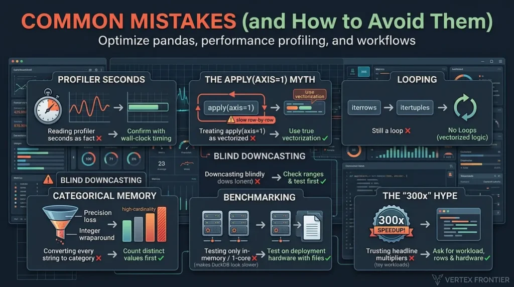
Reading profiler seconds as fact
Profiler timings are inflated and unstable. Compare call counts across runs, then confirm with plain wall-clock timing on the final code.
Treating apply(axis=1) as vectorized
It isn't. It is a per-row Python call, worth about 2 to 4x here, not 100x.
Swapping iterrows for itertuples and stopping
It's a good move, and it's still a loop. Remove the loop.
Converting every string column to category
High-cardinality columns can use as much memory as object, or more. Count distinct values first.
Multiplying the result of map on a categorical
You get a TypeError. Add .astype("float64").
Downcasting blindly
Float32 loses precision, and narrow integers can wrap around on later arithmetic. Check ranges, and leave money alone unless you have tested it.
Comparing engines only on in-memory frames
That setup can make DuckDB look slower than pandas, as our spot-check showed. Test from the file too.
Judging engines on one machine or one sample
Our spot-check ran on a single core, where multithreaded engines can't show their full advantage. Re-run on the hardware you deploy on.
Trusting headline multipliers
"300x" and "1000x" come from specific toy workloads. Ask for the workload, row count, hardware and version.
Benchmarks: Before and After Optimization
| Step | What changed | Result (spot-check, pandas 3.0.6) |
|---|---|---|
| Before | iterrows loop, str columns, 64-bit numbers | 5.7 s at 200,000 rows |
| Fix 1 | Whole-column arithmetic and map | 0.030 s, 192x faster (200,000 rows) |
| Fix 2 | category plus downcast | Vectorized job 0.115 s to 0.032 s (3.5x); memory 70.5 MB to 16.0 MB (1,000,000 rows) |
| After | Same output, checked before timing | Fixes 3 and 4 were not needed for this job |
Same data shape. Same answer. The two fixes ran at different row counts in our test, so we don't multiply them into one headline number. What matters is the order: remove the loop first, then shrink what the remaining code has to touch, and only then shop for engines or hardware.
The Cheapest Matching Rung
Here is the framework that ties the article together. We call it the Cheapest Matching Rung rule:
- Profile the job.
- Find the cheapest rung whose symptom matches your profile.
- Apply that rung only.
- Profile again, because a fix can reveal a different bottleneck underneath.
- Stop as soon as the job is fast enough.
Step 4 is the one people skip. After a loop rewrite, the profile often turns flat, and that flat profile is the signal that the engine question is finally the right one.
Run This on Your Own Data
A benchmark you can't repeat is an anecdote. Use this protocol so your numbers can be trusted, by you and by your team.
- Fix the workload first: the same input, the same output, written down.
- Record versions and hardware: Python, pandas, Polars, DuckDB, CPU cores, RAM.
- Check equality before timing. A fast wrong answer is not a result.
- Do one warm-up run, then time at least five runs and report the median.
- Time both cases: engine handed a DataFrame, and engine handed the file.
- Profile again after each fix, as the Cheapest Matching Rung rule says.
Python Code: a minimal timing helper:
import time import statistics def bench(fn, *args, repeats=5): fn(*args) # warm-up run, not timed times = [] for _ in range(repeats): start = time.perf_counter() fn(*args) times.append(time.perf_counter() - start) return statistics.median(times) print(bench(revenue_vectorized, df))For reference, here is the benchmark card behind this article's own spot-check.
| Field | Our spot-check |
|---|---|
| Workload | Net revenue per order, completed orders only, group by region and channel |
| Rows | 200,000 (loop ladder), 1,000,000 (memory), 3,000,000 (engines) |
| Versions | Python 3.12, pandas 3.0.6, Polars 2.0.0, DuckDB 1.5.6 |
| Hardware | Single-core Linux sandbox |
| Timing | Median of 5 runs after warm-up for engines; fewer runs for the slow loops |
| Correctness | Loop variants checked against the vectorized result |
| Data | Synthetic, randomly generated orders |
Where This Fits in the Wider Data Stack
Pandas performance sits at the crossing of several trends:
- pandas 3.0: the new str dtype and Copy-on-Write defaults change old assumptions about memory and chained operations.
- Polars 2.x and DuckDB 1.5.x: both have moved on since the benchmark. DuckDB's release history and the Polars releases page are the places to check before trusting any ratio.
- Parquet-first workflows: engines shine when they read columnar files. If your files are piling up, migrating Parquet workloads to Iceberg is the next question.
- Statistics code in pandas: loops hide in analysis code too. Our walkthrough of statistical testing workflows in Python shows time-series work where vectorized habits matter.
- Preprocessing pipelines: per-row cleaning is a common offender in data preprocessing pipelines like RAG preparation.
- Analytical databases: when the data outgrows one machine, analytical databases like ClickHouse enter the picture.
The Decision Matrix
Find your symptom, read across, and start at the first row that describes you.
| Symptom | Fix | Expected gain (source) | Main trap |
|---|---|---|---|
Slow loop. Profile full of Series.__getitem__ and isinstance | Rewrite as whole-column operations | 192x in our spot-check at 200k rows; 7.6x if you only switch to itertuples | apply(axis=1) and itertuples are still loops |
| Memory pressure. Swapping, or a MemoryError | Audit, then category and safe downcasts | Whole frame 70.5 MB to 16.0 MB, compute 3.5x (spot-check) | High-cardinality category, float32 precision, map then multiply raising TypeError |
| Flat profile. Reading files dominates | Polars or DuckDB straight from Parquet | 4.7x to 5.9x from Parquet; slower or only 1.8x on in-memory frames (spot-check) | Test from the file, count the learning cost, and re-run on your own cores |
| Tens of GB. Clean code, chosen engine, still an hour | cudf.pandas on an NVIDIA GPU | Up to 150x and 30x (NVIDIA-published, not reproduced here) | Vendor conditions, a GPU requirement, WSL2 memory limits |
Next time pandas feels slow, resist the urge to shop for a new tool. Open a profiler, look at the call counts, and fix the cheapest thing that matches. Then run the protocol above on your own data. Your numbers will differ, and that is exactly why they are the ones to trust.
How We Verified This Article
Every number in this article is labeled by source type. Spot-check figures come from tests we ran on October 10, 2026 and describe on the benchmark card above. NVIDIA figures are attributed to NVIDIA. We read the pandas 3.0 release notes, the pandas categorical and iterrows documentation, both NVIDIA announcements and the current cuDF documentation, and the Garcia, Gross and Quansight posts before citing them. Where we could not verify a figure, we left it out instead of guessing.
Three limits are worth stating. First, GPU results are vendor-published and were not independently reproduced. Second, our spot-check ran on a single CPU core with synthetic data, so treat its ratios as one data point. Third, benchmark ratios are workload-dependent, so treat every multiplier here as a range for planning, not a guarantee. If you find an error, we want to hear about it.
FAQ: Why Pandas is So Slow
Why is pandas so slow compared to Polars or DuckDB?
Often it is not the library. A per-row Python loop is slow in any library. In our spot-check, rewriting the loop was worth about 190x, while on 3 million rows Polars beat in-memory pandas by only 1.8x and DuckDB was 2.4x slower. Both engines were 4.7x to 5.9x faster when they read a Parquet file themselves.
Is iterrows really that slow? What should I use instead?
Yes. It builds a Series for every row, and the pandas documentation notes that it does not preserve dtypes across rows. Use whole-column operations first. If you truly need a loop, itertuples is faster, about 7.6x in our spot-check, but vectorization was worth roughly 190x.
Can pandas handle 10 million rows?
Yes. In our spot-check the vectorized job processed 1 million rows in about 0.11 seconds on one core, and Marc Garcia processed about 120 million records on a 16 GB laptop by reading one year at a time, with a peak near 900 MB. The limit is usually memory and read strategy, not row count.
How do I reduce pandas memory usage without changing my results?
Measure with memory_usage(deep=True), or run an audit that tests the category conversion per column. Convert columns with few distinct values to category, and check ranges before downcasting integers. Downcasting floats to float32 changes precision, so skip it for money. On pandas 3 with PyArrow installed, strings already use less memory, so measure before you convert.
Why does mapping on a categorical column raise a TypeError when I multiply?
map on a categorical column returns a categorical, and the pandas documentation says arithmetic on categorical data raises a TypeError. Add .astype("float64") after the map and the multiplication works. The exact error wording differs between pandas versions.
When is switching to Polars or DuckDB actually worth it?
When your profile is flat, your code is already vectorized, and the job reads Parquet or CSV files. Test from the file, not from a DataFrame pandas already built. Also weigh the learning cost: Polars needs its expression API and DuckDB needs SQL.
Does running pandas on a GPU (cuDF) require rewriting my code?
According to NVIDIA, no. You load the cudf.pandas extension in a notebook or run python -m cudf.pandas on the command line, and your pandas import stays as it is. You do need an NVIDIA GPU. Supported operations run on the GPU and the rest fall back to the CPU. NVIDIA's speedups are vendor-published and were not independently reproduced here.
How do I know which bottleneck my pandas code actually has?
Profile it with cProfile and sort by call count. A flood of Series.__getitem__ and isinstance calls means a row loop. A flat profile points to the engine. Memory pressure points to dtypes, and heavy file reading points to the read layer.
📋 Article Timeline & History
Successfully updated on October 15, 2026 with the latest details.
This article was originally published on October 11, 2026.

Was this article helpful?








[…] Part of that gap, however, is self-inflicted on the Pandas side. In one independent spot-check, once the Pandas code was vectorized and its dtypes tightened, Polars was only 1.8x faster in memory and 4.7x to 5.9x faster when reading Parquet, so tuning Pandas first changes the size of the engine gap. The four fixes are ranked from free to expensive in our Pandas performance breakdown. […]
[…] A strong follow-up point: if you stay in pandas for the local case, the read strategy usually decides the outcome. Chunked reads, selecting only the needed columns, and compact dtypes are what let a 16 GB laptop process roughly 120 million CSV rows, and the full benchmark ladder is in our guide to why pandas is slow. […]