

A one-trillion-parameter model is roughly 2 TB of weights. The biggest accelerators on sale today carry 288 GB each.
That gap is the whole story. Kimi K2 has about 1.04 trillion parameters, which is around 2.1 TB at 16-bit precision. NVIDIA’s Blackwell Ultra B300 and AMD’s Instinct MI355X both top out at 288 GB of HBM3e per GPU. One GPU is not close.
Here is the twist most explainers skip. Picture a server with eight of those 288 GB cards. That is 2,304 GB, so the 2.1 TB of weights would fit with about 220 GB to spare. On paper, problem solved. In production, that server would serve almost nobody, because every active conversation needs its own working memory on top of the weights. Fitting the model is the floor, not the finish line.
So there is no mega computer behind the chatbot you use. There is a coordinated fleet of GPUs, with software deciding which GPU holds what, who talks to whom, and where each request goes. That system is called distributed inference.
This guide gives you a mental model (three constraints), the five techniques that solve them, real numbers from DeepSeek, Meta, Moonshot AI and others, four working calculators, a worked sizing example, a pre-deployment checklist, a glossary, the mistakes practitioners keep making, and a decision helper you can use on your own workload. If you are still deciding whether you need any of this, start with our breakdown of when running AI locally actually makes sense.
Key takeaways
Click any point to expand or collapseThree constraints rule serving
Weights must fit, the KV cache keeps growing, and many users arrive at once.
Every technique solves one constraint
And charges a communication price. Pick by price, not by popularity.
Put the chattiest traffic on the fastest link
Tensor parallelism is happiest on NVLink. Across servers, test before you assume: vLLM measured a 6.6x gap without InfiniBand and none with it.
Weights are paid once. KV cache is paid per user
At 128K context, one sequence on a 405B-class model needs roughly 68 GB.
Splitting prefill from decode only pays
When the KV handoff between pools is fast.
Escalate one rung at a time
More GPUs do not automatically mean more speed.
How to read the numbers in this article
Not every number deserves the same trust. Each figure falls into one of four classes.
| Class | What it means | Examples here |
|---|---|---|
| Vendor claim | A company-run test or marketing figure. Attributed by name, never stated as fact. | NVIDIA Dynamo’s 30x; NVIDIA’s H200 tensor vs pipeline test |
| Paper or first-party report | Authors’ own testbed with stated conditions. Strong evidence for that setup only. | DistServe, Mooncake, Llama 3 paper, vLLM blog posts |
| My arithmetic | Derived from published specs and labeled as such. Correct if the inputs are. | KV cache sizes, weight-memory tables, handoff times |
| User report | A GitHub issue or forum thread about one hardware and version combination. Never universal. | NCCL startup hangs, version regressions |
What Is Distributed Inference?
Distributed inference is the practice of running a trained AI model across multiple GPUs or servers, so that the model’s weights, its working memory and its incoming traffic are shared across devices instead of crammed onto one.
Training builds the model. Inference is the serving half: the model reads a prompt and writes an answer. Distributed inference is what makes that answer arrive in seconds for millions of people at once.
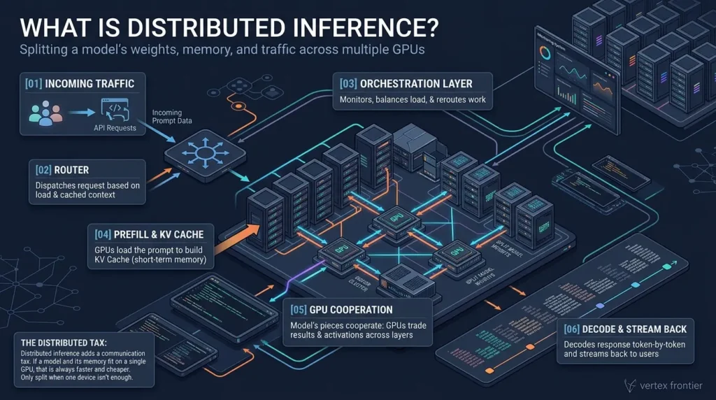
How a request travels, step by step
- A router receives the request: It picks a group of GPUs based on current load, or on which group already holds useful cached context.
- The group runs prefill: It reads the whole prompt in parallel and builds the KV cache, the model’s short-term memory of the conversation.
- The model’s pieces cooperate: Depending on the layout, GPUs hand activations down a line, trade partial results at every layer, or dispatch tokens to specialist sub-networks.
- The group runs decode: It writes the reply one token at a time, reading the KV cache at every step.
- An orchestration layer watches everything: It streams tokens back, balances load, and reroutes work when hardware fails.
Why this matters more every quarter
Serving cost is now the business. Sam Altman wrote in February 2025 that the cost of a given level of AI falls about 10x every 12 months, and usage grows to fill the gap. ChatGPT reported 800 million weekly users in October 2025. NVIDIA’s Jensen Huang said at GTC in March 2025 that reasoning and agentic AI need easily 100 times more compute than the industry expected a year earlier.
The electricity bill follows. The IEA estimates data centres used about 415 TWh in 2024, rising to roughly 945 TWh by 2030, with AI the biggest driver.
Each 10x drop in price per token is earned by engineering. The rest of this article is a tour of that engineering.
Contrarian note: distributed inference is a tax, not a feature. If your model and its working memory fit on one GPU, one GPU per replica is the fastest and cheapest design, because nothing has to talk to anything else. Every technique below exists because that simple design eventually breaks.
Distributed inference splits weights, memory and traffic across devices. Do it only when one device stops being enough.
The Three Constraints Framework
Every serving problem you will debug is one of three problems wearing a costume.
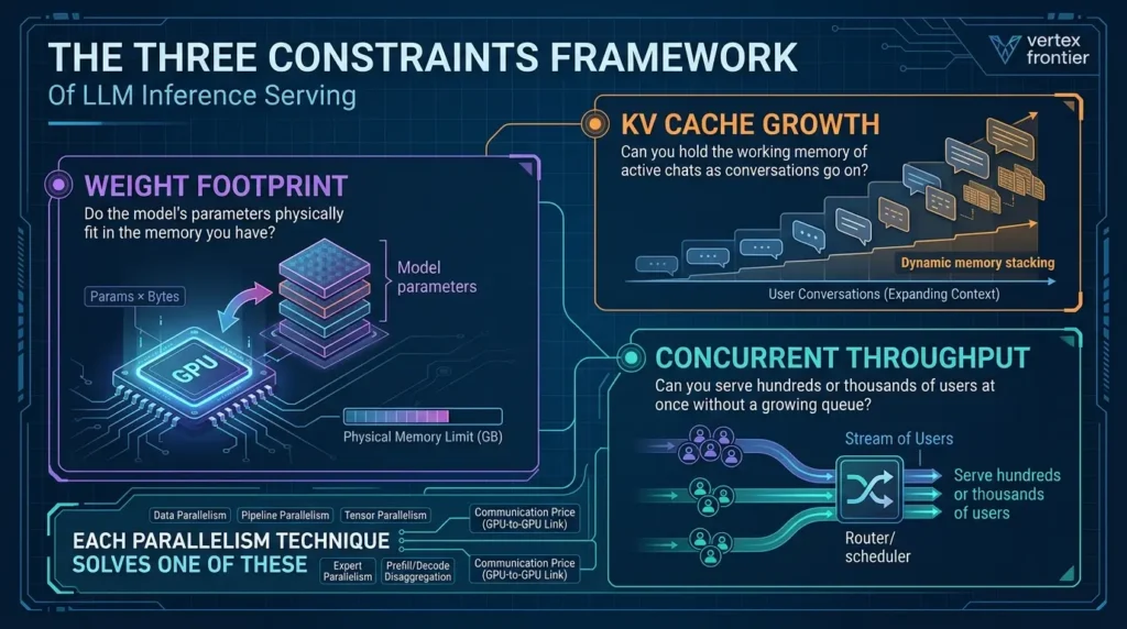
- Weight footprint: Do the model’s parameters physically fit in the memory you have?
- KV cache growth: Can you hold the working memory of every active conversation, which keeps growing as the chat goes on?
- Concurrent throughput: Can you serve hundreds or thousands of users at once without a growing queue?
Each parallelism technique answers one of these. Each also charges a different price in GPU-to-GPU communication. That price list is the part most guides leave out.
| Technique | Constraint it solves | Communication price |
|---|---|---|
| Data parallelism (replicas) | Throughput | None between replicas. Only routing. |
| Pipeline parallelism | Weight footprint | Activations handed from stage to stage |
| Tensor parallelism | Weight footprint, plus lower latency | A blocking all-reduce inside every layer |
| Expert parallelism | Weight footprint for MoE models | All-to-all dispatch and combine at every MoE layer |
| Prefill/decode disaggregation | Interference between two kinds of work | One bulk KV cache transfer per request |
What the hardware gives you
Memory per GPU sets the starting point. These are vendor-listed figures, so treat them as specs, not benchmarks.
| GPU | Memory | Memory bandwidth | GPU-to-GPU link |
|---|---|---|---|
| NVIDIA H100 SXM | 80 GB HBM3 | 3.35 TB/s | NVLink, 900 GB/s |
| NVIDIA H200 | 141 GB HBM3e | 4.8 TB/s | NVLink, 900 GB/s |
| NVIDIA B200 | about 180 GB (datasheet: 1,440 GB across 8 GPUs) | 8 TB/s per GPU | NVLink, 1.8 TB/s |
| NVIDIA B300 | 288 GB HBM3e | about 8 TB/s | NVLink, 1.8 TB/s |
| AMD Instinct MI355X | 288 GB HBM3E | 8 TB/s | Infinity Fabric |
The 288 GB tier arrived in 2025. The H200 and B200 still make up a lot of deployed hardware, and B200 figures vary by source (180 to 192 GB), so check the data sheet for the exact system you buy.
Fit is the floor
Weight memory is simple arithmetic: parameters times bytes per parameter. The numbers below are my calculations from the published parameter counts of Llama 3.1 405B, DeepSeek-V3 and Kimi K2.
| Model | BF16 (2 bytes) | FP8 (1 byte) | FP4 (0.5 byte) |
|---|---|---|---|
| Llama 3.1 405B | about 810 GB | about 405 GB | about 203 GB |
| DeepSeek-V3 (671B) | about 1.34 TB | about 671 GB | about 336 GB |
| Kimi K2 (1.04T) | about 2.1 TB | about 1.04 TB | about 520 GB |
Try 405 at BF16 on 80 GB cards and you get 13 GPUs at the minimum. That is why Meta serves Llama 3.1 405B in BF16 across 16 GPUs on two machines, a case we will unpack shortly.
Now flip it. DeepSeek-V3 in FP8 is about 671 GB. Eight H200s hold 1,128 GB, so the weights fit on one server with about 457 GB left over. Yet DeepSeek runs its decode stage on 320-GPU units. Why would anyone use 40 times more GPUs than the weights need? Because constraint three, throughput, sets the real size once fit is satisfied. Keep that in mind for the DeepSeek case study later.
Fit sets the minimum cluster. Traffic and memory growth set the real one.
Splitting the Weights: Pipeline and Tensor Parallelism
Two techniques split one model across GPUs. One cuts it into layers. The other cuts every layer into slices. They have opposite personalities.
Pipeline parallelism: the assembly line
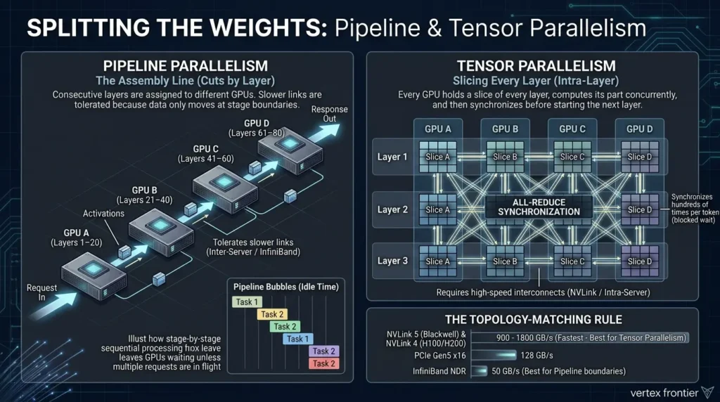
A model is a stack of layers. Pipeline parallelism assigns consecutive layers to different GPUs. Layers 1 to 20 live on GPU A, layers 21 to 40 on GPU B, and so on. A request flows through the stations in order.
The traffic is light. Only the activations at each boundary move, once per stage. That is why pipeline parallelism tolerates slower links, including links between servers.
The catch is idle time. Send one request and only one station works while the others wait. The fix is the same as in a factory: keep many requests in flight. GPipe’s authors measured the idle “bubble” as (K minus 1) divided by (M plus K minus 1), where K is the number of stages and M the number of micro-batches. They found the overhead negligible once M reaches about four times K.
Four stages with four requests in flight leave about 43% of the pipeline idle. Sixteen requests in flight cut that to about 16%. Thirty-two cut it to about 9%.
Two honest caveats. First, GPipe measured this in training, so the formula is an idealized model. For serving, Meta’s Llama 3 paper says pipeline bubbles are not the same concern, because inference has no backward pass and no pipeline flush. Meta still used micro-batching: in a test with two micro-batches (4,096 input tokens, 256 output tokens), throughput improved at the same local batch size. Keeping stages fed still matters.
Second, pipeline parallelism is not just a “fit” tool, and it is not just slow. NVIDIA’s measurements on eight H200 GPUs (Llama 3.1 405B, FP8, TensorRT-LLM, a vendor test) show the split. At concurrency 1, tensor parallelism was 5.6x faster (56 versus 10 tokens per second). At maximum concurrency, pipeline parallelism delivered 1.5x more throughput (764 versus 506). In short: tensor parallelism buys latency, pipeline parallelism buys throughput at lower communication cost. Which wins depends on your latency target and your interconnect.
Tensor parallelism: slicing every layer
Tensor parallelism cuts each layer into slices. Every GPU holds a slice of every layer, computes its piece, then all GPUs combine their partial results before the next layer starts.
That combining step is a collective operation called an all-reduce, and it blocks. Nobody moves on until everyone has contributed. Megatron-LM’s paper counts two all-reduces in the forward pass of each transformer layer (four with the backward pass in training).
Do the arithmetic for a model with 126 layers, like Llama 3.1 405B. Serving it with tensor parallelism means about 252 synchronization points for every token generated. Each one sits on the critical path.
When the links are fast, the payoff is real. Megatron-LM trained an 8.3B-parameter model on 512 GPUs at 76% scaling efficiency. When the links are slow, tensor parallelism can stall. vLLM’s Llama 3.1 test on 16 H100 GPUs (synthetic load, about 1,024 tokens in and 128 out, published in July 2024 as an early reference) measured the gap. Without InfiniBand between the two servers, tensor parallelism 8 plus pipeline parallelism 2 was 6.6x faster than 16-way tensor parallelism. With InfiniBand, the two layouts performed about the same. The Mooncake paper makes the same point from the other side: stretching tensor parallelism beyond one 8-GPU node needs two expensive RDMA all-reduces per layer.
The topology-matching rule
This is the idea that ties the section together: parallelism choice is really a bandwidth-matching decision. Put the chattiest traffic on the fattest link.
Read the chart as a price list. Tensor parallelism pays all-reduce costs hundreds of times per token, so it is safest on the top two bars. Pipeline parallelism pays once per stage boundary, so it tolerates the bottom bar better, though NVIDIA notes that stage-to-stage bandwidth still matters for throughput. With InfiniBand-class links, vLLM measured little difference between the two layouts, so treat this as a default, not a law.
DeepSeek hit the same asymmetry on its H800 cluster, where NVLink delivered about 3.2 times the bandwidth of InfiniBand. Its answer was to cap each token’s expert routing at four nodes.
Note: the rule is about the NVLink domain, not the physical box. NVIDIA’s GB200 NVL72 links 72 GPUs in one NVLink domain, so the safe zone for tensor-style traffic is much bigger on that hardware. Check what your system actually connects.
Case study 1: Meta serves a 405B model across two machines
The challenge. Llama 3.1 405B weighs about 810 GB in BF16, more than the 640 GB on one eight-GPU H100 server. Meta needed to serve it to its own apps.
What they did. According to the Llama 3 paper, Llama 3 405B in BF16 does not fit in one machine with eight H100 GPUs, so Meta serves it across 16 H100 GPUs on two machines. Tensor parallelism runs inside each machine over NVLink. Pipeline parallelism connects the two machines, where bandwidth is lower and latency higher. Meta also built an FP8 version, quantizing most feed-forward layers while keeping self-attention at higher precision.
The result. This section of the paper reports topology, precision and a micro-batching test, not fleet throughput, so there is no production speed number to quote. By my arithmetic, 16 H100s with 80 GB each hold 1,280 GB, which leaves about 470 GB beyond the BF16 weights for KV cache and working space.
The lesson. Meta’s FP8 work also contains a warning. Standard benchmarks showed the FP8 model on par with BF16, yet it occasionally produced corrupted responses when scaling factors were not bounded. Meta switched to checking reward-model score distributions across 100,000 responses. Aggregate benchmark scores can hide rare failures, so validate low-precision serving on output distributions.
Pipeline parallelism lets a model fit. Tensor parallelism makes it fast, but only on fast links. Match each to the wire it will live on.
The KV Cache: Working Memory That Never Stops Growing
Weights are the part everyone remembers. The KV cache is the part that breaks production.
The KV cache is the memory a model keeps of the conversation so far. For every token already processed, the model stores that token’s attention keys and values on the GPU, so it never has to recompute them when generating the next token.
The cache grows with every token, and each concurrent user gets their own. As the vLLM team put it at launch, managing the KV cache efficiently is a significant challenge.
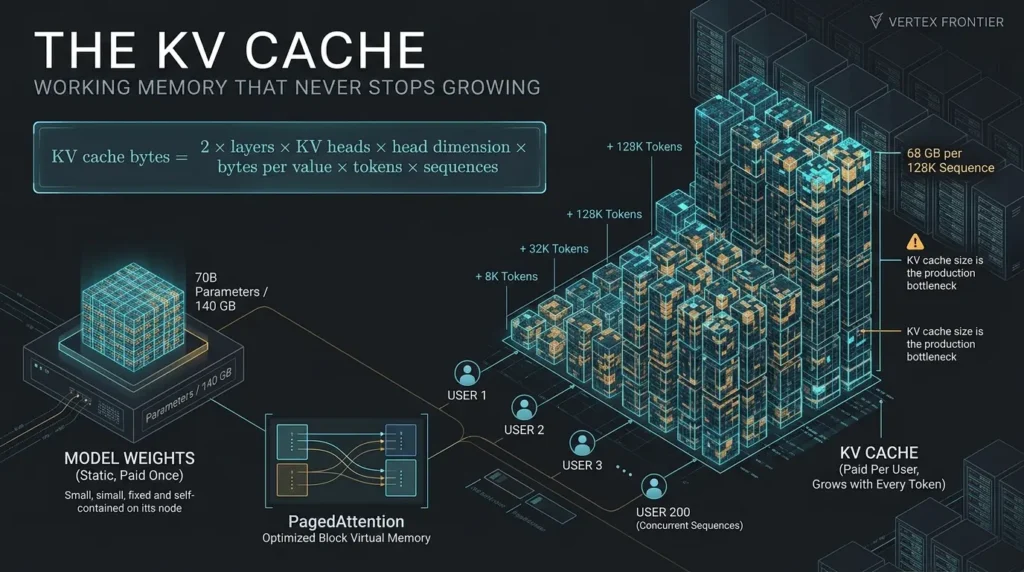
The formula, and why it surprises people
Here is the arithmetic for two real architectures. The layer and head counts come from the Llama 3 paper. The results are my calculations.
| Model (BF16 cache) | Cache per token | One 8K sequence | One 32K sequence | One 128K sequence |
|---|---|---|---|---|
| Llama 3.1 70B | about 328 KB | about 2.7 GB | about 10.7 GB | about 43 GB |
| Llama 3.1 405B | about 516 KB | about 4.2 GB | about 16.9 GB | about 68 GB |
One 128K-token conversation on a 405B-class model eats about 68 GB, roughly 85% of an H100’s 80 GB, before a single weight is loaded. Put 100 users at 8K context on the 70B model and the cache alone is about 268 GB, more than three H100s.
This is the sentence to remember: weights are paid once, but the KV cache is paid per user. That is why the cache, not the weights, usually caps how many people one deployment can serve. Dig into the quality side of this in our piece on context rot, and see how it shows up in agent design in why agent memory architecture is becoming the real production bottleneck.
Worked example: sizing a 70B chat service
Say you want to serve Llama 3.1 70B to 200 users at the same time, each holding up to 8K tokens of context. This is a worst case: every user sits at the full 8K at once. Treat it as a planning number, not a prediction.
The weights are 70 billion parameters times 2 bytes, so about 140 GB at BF16 and 70 GB at FP8. The KV cache is about 328 KB per token (80 layers, 8 KV heads, head dimension 128, from the Llama 3 paper). That is about 2.7 GB per 8K sequence, and about 537 GB for 200 of them. An FP8 cache halves that to about 268 GB; vLLM supports FP8 for the KV cache on recent GPUs.
| Scenario | Weights | KV cache (200 x 8K) | Total | H100 80 GB: needed → GPUs | H200 141 GB: needed → GPUs |
|---|---|---|---|---|---|
| BF16 weights, BF16 cache | 140 GB | 537 GB | 677 GB | 10.6 → 11 | 6.0 → 7 |
| FP8 weights, BF16 cache | 70 GB | 537 GB | 607 GB | 9.5 → 10 | 5.4 → 6 |
| FP8 weights, FP8 cache | 70 GB | 268 GB | 338 GB | 5.3 → 6 | 3.0 → 4 |
How to read the last two columns: “needed” is total memory divided by the usable memory per GPU, after keeping 20% free for runtime and activations (my assumption, the same default as the calculators above). The second number rounds up. Two rows land within 0.1% of a whole GPU, so treat 6 versus 7 and 3 versus 4 as one decision: add headroom. You may also need to round up again to a size your engine supports.
Three lessons fall out of the arithmetic:
- The cache is the bigger bill: In this scenario the KV cache is about 3.8 times the weights.
- Quantize the right thing: Moving the weights to FP8 saves 70 GB. Moving the cache to FP8 saves about 268 GB.
- Concurrency, not model size, drives the cluster: Halve the users and the cache halves too. The weights do not move.
Note: this is a lower-bound sketch. It ignores activation memory, fragmentation, per-GPU imbalance and any rule your engine has about how many GPUs a model can be split across. It also assumes every user holds a full 8K context at once. Real traffic rarely does, which is where paged cache management earns its keep. Validate with the benchmark protocol later in this article.
Architects fight back: GQA and MLA
Model designers know this. Llama 3 uses grouped-query attention with 8 key-value heads to shrink the cache. DeepSeek went further with Multi-head Latent Attention. The DeepSeek-V2 paper reports a 93.3% KV cache reduction.
Using the V3 design, which caches a 576-element latent per token per layer across 61 layers, I get roughly 70 KB per token at 16-bit storage. That is about seven times less than Llama 3.1 405B. Production systems may store it differently, so treat that as a rough comparison, not a benchmark.
One side effect is worth knowing. The vLLM team found that tensor parallelism is not optimal for DeepSeek’s latent attention because the latent projections get duplicated across shards. Model architecture and parallelism choice are coupled.
PagedAttention and the myth it created
Early serving systems reserved memory for each sequence’s worst-case length. The vLLM team reported that existing systems wasted 60% to 80% of KV memory through fragmentation and over-reservation. PagedAttention borrowed an idea from operating systems: store the cache in small blocks, mapped through a table, like virtual memory pages. Waste fell below 4%.
The launch benchmarks (LLaMA models on A100 GPUs) showed up to 24 times the throughput of HuggingFace Transformers and 2.2 to 2.5 times that of TGI in the main setup, and up to 3.5 times in another. Those are 2023 numbers against specific baselines. The peer-reviewed SOSP paper reports 2 to 4 times over FasterTransformer and Orca at the same latency.
Now the myth. Many people believe vLLM lets big models run on small hardware. It does not. The vLLM author said in the launch discussion on Hacker News that it optimizes throughput and does not lower the minimum resources needed to run a model. Paging gives you more users per GPU. It does not shrink the weights.
Case study 2: vLLM turns a memory trick into the industry default
The challenge. KV cache memory is huge, dynamic and wasteful. Fragmentation capped batch sizes, which capped throughput.
What they did. A UC Berkeley team built PagedAttention with block tables, copy-on-write sharing and prefix reuse, then wrapped it in the vLLM engine, first used to serve LMSYS’s Vicuna and Chatbot Arena.
The result. Waste dropped from 60 to 80% to under 4%, and throughput rose by the margins above. NVIDIA describes Dynamo as supporting all major inference backends, which is how a memory technique from 2023 ended up underneath the newest orchestration layers.
The lesson. One systems idea, treating memory like an operating system treats pages, became the base layer of the serving industry. Memory management, not raw FLOPs, is where serving gets won.
Compute the KV cache for your target context and user count first. It decides your batch size, and your batch size decides your cost.
Handling Traffic: Data Parallelism and Smart Routing
Say the model and its cache fit on one GPU, but a thousand people want answers at once. Copy the whole model onto several GPUs and route each request to one of them. That is data parallelism.
Replicas never talk to each other. You are only deciding which door each request walks through. That makes it the cheapest technique in communication terms and the easiest to operate.
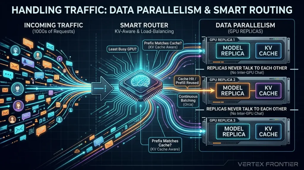
Routing is where the cleverness lives
A router can send work to the least busy replica. A smarter one sends it to the replica that already holds the cached prefix of the prompt, so prefill work is not repeated.
SGLang’s RadixAttention reuses KV cache across requests with a radix tree and reports up to 6.4 times higher throughput across agent, reasoning and multi-turn workloads. NVIDIA Dynamo ships a KV-aware router for the same reason. This matters more as agents resend long, repeated prompts. If you build agents, this trade-off lands on your desk fast, because agent loops resend long, repeated prompts all day.
Batching is the other traffic lever. The Orca paper introduced iteration-level scheduling, letting new requests join a running batch between token steps. On GPT-3 175B it reported 36.9 times the throughput of NVIDIA FasterTransformer at the same latency. Continuous batching is now standard in modern engines.
Contrarian note: “just add replicas” quietly burns money. Each replica carries a full copy of the weights, so every extra copy spends memory on duplicates instead of on KV cache. Past a point, a better layout (or cache-aware routing) serves more users per dollar than another copy of the same model.
Data parallelism solves traffic with zero GPU-to-GPU chatter. Make the router smart before you make the fleet bigger.
Mixture of Experts and Expert Parallelism
A dense model runs every weight for every token. A mixture-of-experts (MoE) model holds many smaller sub-networks, called experts, and a router picks a few for each token.
DeepSeek-V3 has 671 billion parameters but activates about 37 billion per token. Its layers use 256 routed experts plus one shared expert, and each token goes to eight of the routed ones. Kimi K2 goes further, with 384 experts and about 32 billion active parameters out of roughly 1.04 trillion.
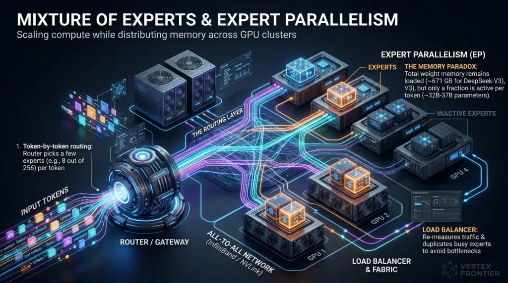
The memory paradox
Active parameters cut compute per token. They do not cut memory. Every expert has to be loaded, because the router could pick any of them for the next token. DeepSeek-V3 touches about 37 billion parameters per token, yet its FP8 weights still take about 671 GB.
Serving cost therefore follows total parameters for memory and active parameters for compute. Headlines quoting only active parameters undersell what the cluster needs.
What expert parallelism does
Expert parallelism spreads the experts across GPUs, so each GPU holds a slice of the experts instead of a copy of the whole model. At every MoE layer, each token is dispatched to the GPUs holding its chosen experts, and the results are combined afterward.
That dispatch and combine is an all-to-all exchange, and it is the communication price. DeepSeek manages it deliberately. Its technical report describes sending each token to at most four nodes and using NVLink inside nodes after the InfiniBand hop. In its decode stage, each GPU hosts one expert across a 320-GPU unit, with extra GPUs holding redundant copies of hot experts.
The open-source side is converging on the same design. vLLM’s Wide-EP work combines expert and data parallelism with dual-batch overlap, which hides communication behind compute, and an expert load balancer. The team reports a sustained 2,200 tokens per second per H200 on a CoreWeave cluster with InfiniBand. That is a vendor-side benchmark for DeepSeek-style models on that hardware, not a universal figure.
Load balance is the hard part
If one expert gets far more tokens than the others, its GPU becomes the bottleneck for the whole layer. This is why vLLM’s expert-parallel documentation includes an expert-parallel load balancer, and why DeepSeek re-measures expert load from live traffic and duplicates the busiest experts.
MoE saves compute, not memory. Expert parallelism trades that compute saving for all-to-all network traffic, so it needs a serious fabric.
Splitting Prefill from Decode: Disaggregation
One request has two very different lives.
Prefill/decode disaggregation is the practice of running the two phases of inference, reading the prompt (prefill) and writing the answer (decode), on separate pools of GPUs, each tuned for its own bottleneck.
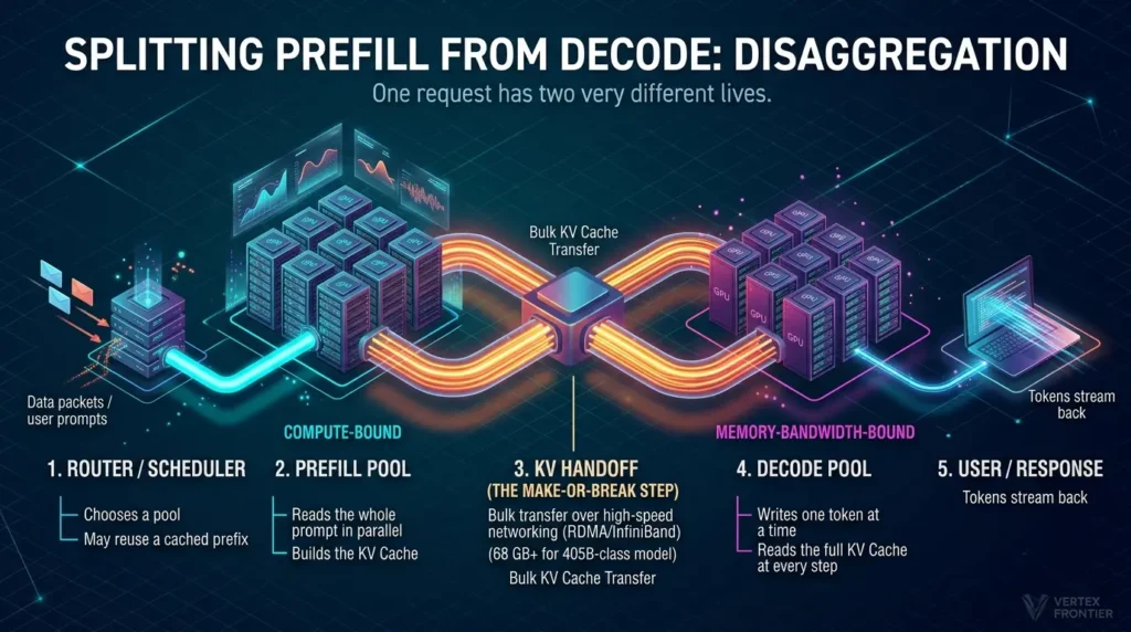
Two phases, two bottlenecks
- Prefill reads the whole prompt in parallel. It is compute-bound, and it builds the KV cache.
- Decode writes one token at a time and reads the full KV cache at every step. It is memory-bandwidth-bound, and its memory need grows as the answer grows.
Put both on the same GPUs and they fight. A long prompt arriving mid-conversation can stall the token streams of other users. The DistServe paper frames this with two latency targets: time to first token (TTFT) for prefill, and time per output token (TPOT) for decode. Colocated systems must favor one or overprovision.
The metric that matters is goodput, the request rate you can serve while meeting both targets. For a practical guide to measuring it, see how to benchmark long-context models properly. The latency pressure from long contexts is also the theme of our guide to recursive language models.
What the papers report
These are results from specific testbeds. Read them as “what is possible,” not “what you will get.”
| System | Reported result | Conditions |
|---|---|---|
| DistServe | Up to 7.4x more requests, or 12.6x tighter latency targets | Versus colocated systems, in the authors’ testbed. An earlier abstract said 4.48x and 10.2x. |
| Splitwise | 1.4x throughput at 20% lower cost, or 2.35x throughput at the same cost and power | Microsoft Research, phase-split machines |
| Mooncake | Up to 525% more throughput in simulated scenarios; about 75% more requests in a replay of real Kimi traces | Same latency targets. Dummy model with LLaMA2-70B architecture on A800 GPUs; vLLM baseline. Later journal version reports different figures (see note). |
A note on versions. Papers get revised, and the numbers move. DistServe’s early arXiv abstract said 4.48x and 10.2x, while the OSDI ’24 version says 7.4x and 12.6x with more than 90% of requests inside the latency targets. Mooncake’s July 2024 arXiv abstract gives the 525% and 75% figures above, while the later journal abstract (ACM Transactions on Storage, as listed on the Tsinghua group’s publication page) reports 59% to 498% more effective request capacity on real traces, and 115% and 107% more requests on A800 and H800 clusters. Same system, different test sets and dates. Quote the version you actually read.
The handoff decides everything
Disaggregation adds a step. The whole KV cache must travel from the prefill pool to the decode pool before the first token can appear.
Chooses a pool. May reuse a cached prefix.
Reads the whole prompt in parallel. Compute-bound. Builds the KV cache.
Bulk transfer over RDMA-class networking. The make-or-break step.
Writes one token at a time. Memory-bandwidth-bound.
Tokens stream back.
Do the math for the earlier example. A 128K-token cache on a 405B-class model is about 68 GB. Moving that over one 50 GB/s InfiniBand port takes about 1.4 seconds at perfect line rate. Over a 100 Gb/s Ethernet link (12.5 GB/s) it takes about 5.4 seconds. Over 900 GB/s NVLink it takes under 0.1 seconds.
Real systems do better than a single-link estimate by spreading traffic over several network cards and streaming the cache layer by layer while prefill is still running. Mooncake does exactly that. Still, the order of magnitude explains why the handoff needs dedicated, RDMA-class networking, and why Mooncake moves KV cache over RDMA. Plain TCP over ordinary Ethernet is usually not fast enough to make the split worth it.
When not to split
Disaggregation is not a free upgrade. Mooncake’s own paper says the case for a separate prefill pool is still debated now that chunked prefill exists, and the authors explain why they kept disaggregation anyway. Skip it when:
- your prompts are short and decode and prefill rarely collide,
- your cluster is small, so two pools mean two half-empty pools,
- you lack RDMA-class networking between nodes,
- your latency targets are loose enough that colocation already meets them,
- chunked prefill, the main alternative, already keeps your decode latency inside target. Test it first.
Measure interference first. If your TTFT and TPOT targets hold, you do not need this.
Case study 3: Mooncake rescues Kimi from overload
The challenge. Moonshot AI’s Kimi faced constant overload. In the Mooncake paper, long prompts on shared GPUs wrecked decode latency, and idle CPU memory and SSDs sat unused across the cluster.
What they did. They split prefill and decode into separate clusters, built a global scheduler, and created a KV cache pool that spans GPU memory, CPU DRAM and SSD, moved over RDMA. They also added prediction-based early rejection: under overload, refuse a request the system cannot serve within its targets instead of letting everyone queue.
The result. In the paper’s simulated long-context scenarios, throughput rose by 50% to 525% under the same latency targets. On a replay of real request traces (10 prefill plus 10 decode instances against 20 vLLM instances; time-to-first-token limit 30 seconds, time-between-tokens limit 0.1 seconds), Mooncake handled about 75% more requests, and about 100% of its requests met the token-latency limit against 57% for the vLLM baseline. One condition matters: to protect proprietary details, the experiments used a dummy model with LLaMA2-70B’s architecture on A800 GPUs, not Kimi’s production model.
The lesson. The real cost of not disaggregating is not a slower average. It is the failing tail, the share of users who miss the latency target. And treating the KV cache as a cluster-wide, multi-tier resource bought more than any single-GPU trick.
Split prefill from decode when the two phases measurably hurt each other, and only with a fast handoff between pools.
Putting It All Together: Multi-Dimensional Parallelism
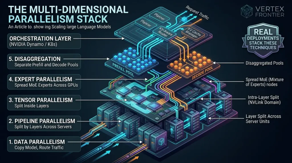
Real deployments stack these techniques. The five in one list:
- Data parallelism: copy the model, route the traffic.
- Pipeline parallelism: split by layers, usually across servers.
- Tensor parallelism: split inside layers, usually within one NVLink domain.
- Expert parallelism: spread MoE experts across GPUs.
- Disaggregation: give prefill and decode their own pools.
Stacked together, this is multi-dimensional parallelism. Each layer of the stack is matched to the link it can afford.
The orchestration layer
On top of the GPUs sits a control layer that routes requests, balances load, scales pools up and down, and survives failures without dropping requests. If you build harnesses around models, the reliability patterns will look familiar. We cover them in how production harnesses handle retries and circuit breakers.
NVIDIA Dynamo packages this layer as open source. NVIDIA describes four parts: a planner that moves GPUs between prefill and decode, a KV-aware router, a KV cache manager that offloads across memory tiers, and a low-latency transfer library called NIXL. It sits above vLLM, SGLang and TensorRT-LLM rather than replacing them.
NVIDIA’s own numbers come with fine print. For DeepSeek-R1 on GB200 NVL72, the launch blog reports disaggregated serving increasing the requests served by up to 30 times, using layouts it lists (for example context EP4/DP16 and generation EP64/DP3). For Llama 70B on Hopper it reports more than 2 times. NVIDIA also words the headline differently across its own pages: requests served in the blog, throughput per GPU on the Dynamo product page, and tokens per GPU in the launch press release. These are vendor claims from vendor tests, and the metric is not identical in every statement.
Practitioners are less starry-eyed. One engineer’s comment on the Dynamo launch thread said that after a year of trying to get various NVIDIA inference products working, the advice was simply “beware.” Others in the thread praised the design. The honest read is that vendor stacks are powerful and demanding, and you should test them on your own workload. Part of the problem is cultural: a commenter noted that nobody publishes apples-to-apples engine benchmarks anymore, because someone always objects to the version or patch used.
Related concepts worth knowing: quantization (FP8 and FP4) cuts both weight and cache memory. Speculative decoding speeds up the decode phase. Cache layers such as LMCache extend the KV cache beyond GPU memory. Kubernetes-based stacks like llm-d and Ray Serve handle deployment. Each sits next to the techniques above, not instead of them.
Case study 4: DeepSeek serves a 671B model on a tight budget
The challenge. Serve V3 and R1 to a huge global audience on H800 GPUs, at prices far below Western rivals, while meeting online latency targets. MoE sparsity makes per-GPU batches tiny unless many nodes batch together.
What they did. All of the following comes from DeepSeek’s V3 technical report and its inference-system overview.
- Prefill and decode run in separate pools. The V3 report (December 2024) describes a minimum prefill unit of 32 GPUs and a minimum decode unit of 320 GPUs, with expert parallelism spanning each. DeepSeek’s later production setup may differ, so read these as the report’s deployment units.
- Communication is overlapped with compute using two micro-batches, so the network hides behind math.
- Three load balancers handle prefill, decode KV cache usage and expert load, with hot experts duplicated.
- The KV cache lives on disk too. DeepSeek announced disk-based context caching in August 2024, and in the measured 24-hour window 56.3% of input tokens were cache hits.
- Nodes serving users by day are reassigned to research and training at night.
The result. Over one 24-hour window (27 to 28 February 2025), DeepSeek reported a peak of 278 H800 nodes (2,224 GPUs) and an average of 226.75 nodes, 608 billion input tokens (342 billion, or 56.3%, served from the on-disk cache), and per-node throughput of about 73.7k input and 14.8k output tokens per second. At an assumed $2 per GPU-hour, the daily cost was $87,072 (226.75 nodes x 8 GPUs x 24 hours x $2). Had every token been billed at R1’s published prices, revenue would have been $562,027, a 545% cost-profit ratio.
The caveat that matters. That 545% is theoretical. DeepSeek’s own post notes that V3’s pricing is significantly lower than R1’s, so billing every token at R1 rates overstates real revenue. TechCrunch’s coverage labeled it theoretical too. Read it as a systems-engineering claim about unit economics, not an income statement.
The lesson. Prices show what cache reuse is worth. In the Day-6 post, R1’s cache-hit input price was $0.14 per million tokens against $0.55 for a miss, roughly a 4x gap. DeepSeek’s current pricing page, retrieved on 12 October 2026, lists deepseek-v4-flash at $0.007 per million cache-hit input tokens against $0.22 for a miss at off-peak rates, about a 30x gap, with off-peak at half the peak rate. Prices change and third-party summaries disagree with each other, so read the page itself before budgeting. Disaggregation, wide expert parallelism and cache reuse together turned a giant MoE into a cheap commodity API. For the launch-era prices, see the R1 release notes.
Production serving is several techniques layered together, each matched to a link, all wrapped in an orchestration layer that earns its keep on failures and load shifts.
Which Technique When: The Escalation Ladder
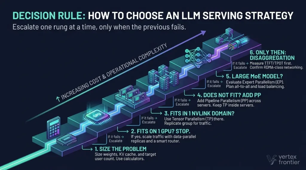
Here is the idea that turns this whole article into a decision rule. Escalate one rung at a time, and only when the previous rung fails. Each rung adds communication cost and operational complexity.
How to choose a strategy in six steps
- Size the problem: Use the calculators above to get weight memory and KV cache at your target context length and user count.
- If it fits on one GPU, stop: Scale traffic with data-parallel replicas and a smart router.
- If it fits inside one NVLink domain, use tensor parallelism there: Replicate the group for traffic.
- If it does not fit, add pipeline parallelism across servers: Keep tensor parallelism inside each server and keep enough requests in flight.
- For large MoE models, evaluate expert parallelism: Plan for all-to-all traffic and expert load balancing.
- Only then test disaggregation: Measure TTFT and TPOT first, and confirm RDMA-class networking.
For a feel of what these choices look like in a serving command, here is a sketch for vLLM. The first three lines follow vLLM’s Llama 3.1 announcement (July 2024). The last follows vLLM’s expert-parallel docs. Flags and defaults change between releases, so check the docs for yours.
Shell (vLLM, illustrative):
# One 8-GPU server, dense model too big for one GPU vllm serve <your-model> --tensor-parallel-size 8
Two servers: tensor parallel inside, pipeline parallel across
(needs a multi-node setup such as Ray)
vllm serve  --tensor-parallel-size 8 --pipeline-parallel-size 2
MoE model: attention data parallel plus expert parallel (flags vary by version)
vllm serve  --tensor-parallel-size 1 --data-parallel-size 8 --enable-expert-parallel
Command status matrix. What each line is, and how far to trust it.
| Layout | Source | Date and version | Status |
|---|---|---|---|
| TP 8 on one 8-GPU server (FP8 405B) | vLLM Llama 3.1 announcement | July 2024 | Documented in the blog for 8xH100 or 8xA100. Re-test on your release. |
| TP 8 x PP 2 across two servers (BF16 405B) | vLLM Llama 3.1 announcement | July 2024 | Documented for 16 GPUs on 2 nodes. The blog called performance preliminary. |
| TP 16 across two servers | vLLM Llama 3.1 announcement | July 2024 | Documented. Performed about the same as TP 8 x PP 2 with InfiniBand, much worse without. |
| TP 1 x DP 8 with expert parallel (MoE) | vLLM expert-parallel docs | Current docs page, October 2026 | Documented as an example for a DeepSeek-V3-class model. Version-sensitive. |
None of these lines was run for this article. Treat them as documented starting points, not tested recipes.
Start at the cheapest rung that works. Each step up buys capacity and charges you in network traffic and operational complexity.
Common Mistakes (and How to Avoid Them)
Most of these come from practitioners’ own reports, so treat them as documented experience, not universal laws.
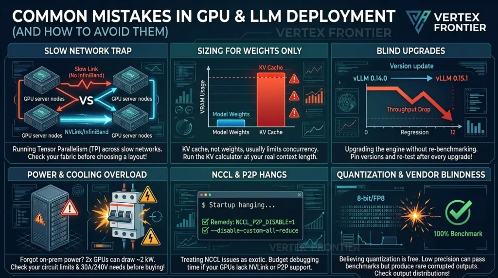
Running tensor parallelism across a slow network
Chatty all-reduces over ordinary links are a classic self-inflicted slowdown. In vLLM’s 16-GPU Llama 3.1 test, TP 8 x PP 2 was 6.6x faster than 16-way TP without InfiniBand, and about equal with it. Check your fabric before you choose a layout.
Choosing tensor or pipeline parallelism without naming your target
In NVIDIA’s H200 test, tensor parallelism won on single-request latency (5.6x) and pipeline parallelism won on maximum throughput (1.5x). Decide whether you are optimizing interactivity or total throughput, and keep enough requests in flight that stages do not idle.
Treating NCCL problems as exotic
A vLLM GitHub issue (vLLM 0.12.0, two RTX PRO 6000 Blackwell GPUs) reports tensor-parallel startup hanging indefinitely unless NCCL_P2P_DISABLE=1 was set. A vLLM forum thread describes a similar hang on PCIe-only Blackwell servers that went away with –disable-custom-all-reduce. These are user reports about specific hardware and versions, not universal behavior. Budget debugging time if your GPUs lack NVLink or peer-to-peer support.
Upgrading the engine without re-benchmarking
A reported regression saw throughput drop between vLLM 0.14.0 and 0.15.1 on specific models under load. Pin versions and re-test after every upgrade.
Believing quantization is a free lunch
Meta’s FP8 experience (above) shows low precision can pass benchmarks and still produce rare corrupted outputs. Check output distributions, not only scores.
Sizing for weights only
The KV cache, not the weights, usually limits concurrency. Run the KV calculator at your real context length.
Quoting vendor benchmarks as if they were yours
Dynamo’s 30x is a vendor figure for one configuration. DeepSeek’s 545% is a theoretical ratio. Neither is a promise about your workload.
Forgetting power and cooling on-prem
One home-lab builder reported 300 W at idle and about 2 kW for two 4090s, enough to flip a breaker, and paid about 600 CAD for a new 30A/240V circuit. A real multi-GPU node needs more. Check the electrical plan before you buy.
Symptom-to-cause map
A quick triage table. Each row names the evidence behind it.
| Symptom | Likely cause | First check | Evidence |
|---|---|---|---|
| Tensor-parallel startup hangs | Peer-to-peer or NCCL problems, reported on PCIe-only GPUs | Try NCCL_P2P_DISABLE=1, check GPU topology and engine version | User reports (vLLM issue and forum thread above) |
| Multi-node tensor parallelism far slower than expected | All-reduce traffic over a slow fabric | Compare TP 8 x PP 2 with TP 16 on your network | vLLM test: 6.6x without InfiniBand |
| Idle GPUs in a pipeline | Too few requests in flight | Run the pipeline calculator, raise concurrency or micro-batches | GPipe formula plus my arithmetic |
| Streaming stalls when long prompts arrive | Prefill and decode interference | Measure TTFT and TPOT, test chunked prefill, then disaggregation | DistServe; Mooncake replay (57% vs about 100% on token latency) |
| Good benchmark scores, rare corrupted outputs | Low-precision serving artifacts | Compare output score distributions, not only averages | Llama 3 paper (FP8 case) |
| Out of memory at long context with few users | KV cache sized wrongly | Run the KV calculator at real context times concurrency | My arithmetic |
Myths and what the evidence says
| Myth | What the evidence says |
|---|---|
| “vLLM lets big models run on small hardware.” | Its author said at launch that it raises throughput but does not lower the minimum resources needed to run a model (launch discussion). |
| “A mixture-of-experts model is small in memory.” | Active parameters cut compute, not memory. DeepSeek-V3 activates about 37B of 671B parameters but still needs every expert loaded (V3 report). |
| “Tensor parallelism must stay inside one server.” | A safe default, not a law. vLLM saw about equal results with InfiniBand and a 6.6x gap without it (vLLM blog). |
| “Pipeline parallelism is only for fitting a model.” | NVIDIA measured 1.5x higher maximum throughput with it, and 5.6x worse single-request latency (NVIDIA H200 test). |
| “Disaggregation always wins.” | Reported gains come from specific testbeds, need a fast KV handoff, and compete with chunked prefill (Mooncake paper). |
Before and After: What Changes When You Get It Right
A before-and-after with real, measured numbers comes from Mooncake’s replay of production-style traffic, and a second comes from straightforward sizing arithmetic.
| Before | After | |
|---|---|---|
| Latency targets (Mooncake replay) | Colocated vLLM baseline met the decode-latency target for 57% of requests | Disaggregated Mooncake met it for nearly all requests |
| Capacity (Mooncake, real workloads) | Baseline capacity | 75% more requests handled |
| Memory (illustrative sizing for Llama 3.1 405B, BF16) | One eight-GPU H100 server: 640 GB of GPU memory against about 810 GB of weights, so it cannot load the model | Two servers, 16 GPUs, 1,280 GB: tensor parallelism inside each, pipeline parallelism between them, about 470 GB left for KV cache |
The first two rows come from the Mooncake paper, measured on a dummy model with LLaMA2-70B’s architecture replaying real request traces, so they show what the design can do, not what you will get. The memory row is my arithmetic, built on Meta’s published topology.
A benchmark protocol you can run
The numbers in this article are other people’s results. Yours will differ. This protocol makes your own numbers defensible. It is a test plan, not a result.
| Field | What to record | Why it matters |
|---|---|---|
| Hardware and fabric | GPU model and count, NVLink, InfiniBand or Ethernet | Topology decided the vLLM and NVIDIA results above |
| Software versions | Engine and version, driver, CUDA, NCCL | vLLM itself called its 2024 multi-node numbers preliminary |
| Model and precision | Parameters, BF16 or FP8, KV cache precision | Precision changes memory and sometimes quality |
| Workload shape | Input and output length distribution, shared-prefix share, arrival pattern | Mooncake’s results depended on trace shape and cache ratio |
| Load | Concurrency sweep or request rate, warm-up, duration | One concurrency point can flip tensor versus pipeline |
| Metrics | TTFT, TPOT, p50, p90, p99, goodput at your target, tokens per second per GPU | Averages hide the failing tail |
| Cache state | Prefix cache on or off, cold or warm | Cache hits change prefill cost dramatically |
| Repeats | At least three runs, report the spread | A single run is an anecdote |
| What it does not prove | Write one sentence | Keeps the result honest |
| Run | Layout (TP/PP/DP/EP) | Concurrency | TTFT p90 | TPOT p90 | Goodput at target | Tokens/s/GPU | Notes |
|---|---|---|---|---|---|---|---|
| 1 | |||||||
| 2 | |||||||
| 3 |
What It Costs: Three Levers
Inference cost comes down to three levers.
- Utilization: Keep GPUs busy with continuous batching and enough requests in flight.
- Reuse: Every KV cache hit is prefill you do not pay for. DeepSeek’s 56.3% hit rate, and a cache-hit price that is 4x lower than a miss for R1 in 2025 and about 30x lower for V4 Flash today, show the size of this lever.
- Idle time: DeepSeek reassigns nodes from serving to research at night, and its pricing page now charges half price off-peak to fill the gap.
Cost per million tokens: do it with your own numbers
Public price lists tell you what vendors charge. Your cost depends on what your GPUs actually deliver. The arithmetic is short.
Three cautions keep the result honest.
- Measure at your latency target: Tokens per second at any latency is not the same as goodput. Use the benchmark protocol above.
- Price one kind of token at a time: Input and output tokens are not interchangeable. DeepSeek’s Day-6 post reports roughly 73.7k input and 14.8k output tokens per second per node, and the input figure includes cache hits. Pick the token type your measurement counts.
- Name your GPU price: DeepSeek’s own analysis assumed a $2 per GPU-hour lease for H800s. Your rate, your commitment term and your power costs will differ.
Money is not the only bill. The IEA’s projection of data-centre electricity roughly doubling by 2030 is the macro version of the power problem a single home-lab owner hits at the breaker.
Pre-Deployment Checklist
Everything above compresses into one pass you can run before a launch. Tick items as you confirm them. Each one points back to a section of this article.
0 of 16 items checked.
A checklist cannot prove your deployment is right. It makes sure the questions that break production were at least asked.
Where This Leaves You
The best distributed inference design is the smallest one that works. Size the weights and the KV cache first. Climb the ladder one rung at a time. Match every technique to the wire it will run on. Measure before you add complexity, and trust your own benchmarks over anyone's headline number.
If you are building on top of served models, the next layer up is agent design. Our guide to production AI engineering concepts picks up where this one stops.
Glossary
The 20 terms used in this article, in plain language. Skim it if a word slowed you down.
| Term | Definition |
|---|---|
| TTFT (time to first token) | The time from a request arriving to the first generated token. Prefill drives it. |
| TPOT (time per output token) | The average gap between consecutive output tokens for one request. Decode drives it. The Mooncake paper calls the same idea time between tokens (TBT). |
| SLO (service level objective) | A latency target you commit to, such as a p90 TTFT or TPOT limit. |
| Goodput | The request rate you can serve while still meeting your latency targets. DistServe defines it per GPU. |
| Prefill | The phase where the model reads the whole prompt in parallel and builds the KV cache. Usually compute-bound. |
| Decode | The phase where the model writes the answer one token at a time, reading the KV cache at every step. Usually memory-bandwidth-bound. |
| KV cache | The stored attention keys and values of every token already processed, kept so they are not recomputed. |
| PagedAttention | Storing the KV cache in small blocks mapped through a table, like virtual memory pages, to cut wasted memory. |
| Continuous batching | Letting new requests join and finished ones leave a running batch between token steps, instead of waiting for a whole batch to finish. The Orca paper calls it iteration-level scheduling. |
| Chunked prefill | Splitting a long prompt into chunks that are mixed into decode batches, so one long prompt does not stall everyone else. |
| Prefill/decode disaggregation | Running prefill and decode on separate pools of GPUs, each tuned for its own bottleneck. |
| All-reduce | A collective operation where every GPU contributes a partial result and every GPU receives the combined sum. Tensor parallelism needs it inside layers. |
| All-to-all | A collective operation where every GPU sends different data to every other GPU. Expert parallelism uses it to dispatch and combine tokens. |
| NVLink | NVIDIA's high-bandwidth GPU-to-GPU interconnect, usually within one server or rack-scale domain. |
| InfiniBand | A high-performance network standard used between servers in GPU clusters. |
| RDMA | Remote direct memory access: network cards move data between the memory of two machines with little CPU involvement. |
| GQA (grouped-query attention) | Several query heads share one set of key-value heads, which shrinks the KV cache. Llama 3 uses 8 KV heads. |
| MLA (multi-head latent attention) | DeepSeek's design that caches a compressed latent per token instead of full keys and values. |
| MoE (mixture of experts) | A model with many sub-networks (experts) where a router picks a few per token. Total parameters set memory, active parameters set compute. |
| Quantization | Storing weights or the cache in fewer bits, such as moving from BF16 to FP8 or FP4, to save memory and bandwidth. |
FAQ
What is distributed inference?
Distributed inference runs a trained AI model across several GPUs or servers. The model's weights, its working memory (the KV cache) and its incoming traffic are shared across devices, so a model too big for one GPU can still serve many users at once.
What is the difference between tensor, pipeline, data and expert parallelism?
Data parallelism copies the whole model to handle more traffic. Pipeline parallelism splits it by layers. Tensor parallelism splits each layer into slices that synchronize at every layer. Expert parallelism spreads a mixture-of-experts model's experts across GPUs. Each one solves a different constraint and has a different communication cost.
How many GPUs do I need to run a 70B model?
The weights alone are about 140 GB at BF16 (70 billion parameters x 2 bytes), so you need at least two 80 GB GPUs before counting any KV cache. At FP8 the weights are about 70 GB. KV cache for many users adds more, so use the calculators in this article with your real context length and concurrency.
What is a KV cache and why does it use so much memory?
The KV cache stores the attention keys and values of every token already processed, so the model does not recompute them. It grows with context length and is kept separately for each concurrent user. By this article's arithmetic, one 128K-token sequence on a Llama 3.1 405B-class model needs about 68 GB.
Does vLLM reduce the memory needed to load a model?
No. PagedAttention reduces waste in the KV cache, which lets a GPU serve more users. It does not shrink the weights. The vLLM author said at launch that the engine improves throughput without lowering the minimum resources needed to run a model.
Does tensor parallelism have to stay inside one server?
It is a safe default, not a law. In vLLM's July 2024 test on 16 H100 GPUs, tensor parallelism 8 plus pipeline parallelism 2 was 6.6x faster than 16-way tensor parallelism when the servers lacked InfiniBand, and the two layouts performed about the same with InfiniBand. Test on your own fabric.
Why is my multi-GPU inference slower than a single GPU?
Usually communication. Tensor parallelism over a slow fabric, a pipeline without enough requests in flight, or peer-to-peer problems at startup can leave GPUs waiting on each other. Match each technique to its link, check the pipeline calculator, and re-benchmark after every engine upgrade.
When is prefill/decode disaggregation worth it?
When long prompts measurably hurt other users' token streaming, your cluster is large enough for two efficient pools, and you have RDMA-class networking for the KV handoff. Test chunked prefill first. If your latency targets already hold on colocated GPUs, the extra complexity is not worth it.

Was this article helpful?




[…] its own, which is one reason long-context requests get routed across multi-GPU fleets, our guide to how distributed inference actually work covers that […]
[…] memory also has a literal hardware footprint: at serving time, every token in the window occupies KV-cache space on a GPU, which is why window size shows up in serving architecture decisions, not just prompt […]