

A seasonal forecast can fail even when the model runs without an error. The code may fit, the residual plot may look acceptable, and the forecast may still miss the business pattern that matters most: next December’s demand, next week’s load, or the next summer peak.
SARIMA helps because it gives a model an explicit seasonal memory. Instead of asking only how recent observations influence the next one, it can also model what happened one complete seasonal cycle ago. But SARIMA is not a magic switch. The seasonal period must be correct, transformations must stay on the same scale, and the final model must beat a simple baseline on forecasts it has not seen.
This guide builds that workflow in Python with statsmodels. It explains the notation, shows how to choose candidate orders without treating ACF and PACF as an oracle, and walks through a leakage-aware implementation with prediction intervals, residual diagnostics, and seasonal-naive comparison.
Key takeaways
Click any topic to expand or collapsePrerequisites and compatibility
The walkthrough assumes a regular, time-ordered series and a CSV with a date column plus one numeric target column. Install the packages used in the examples with:
Bash:
python -m pip install pandas numpy matplotlib scipy statsmodels scikit-learnThe RMSE example uses root_mean_squared_error, which is available in scikit-learn 1.4 and later. Pin the versions used by your notebook or project and rerun the code before publishing; package defaults and warnings can change.
| Requirement | What to verify before fitting | Why it matters |
|---|---|---|
| Time index | Sorted, regular frequency with duplicates and missing periods investigated | Seasonal lags only mean what you think they mean when each step has a stable meaning. |
| Target values | Numeric target; zeros and negative values checked before Box–Cox | The transformation and inverse transformation depend on the data domain. |
| Forecast horizon | Defined before tuning, such as 12 months or 7 days | A model can be useful at one horizon and weak at another. |
| Baseline | Naive and seasonal-naive forecasts prepared on the same splits | Complexity is justified only when it adds measurable value. |
What is SARIMA?
SARIMA stands for Seasonal AutoRegressive Integrated Moving Average. It is an extension of ARIMA for a univariate time series with a repeating seasonal structure.
A non-seasonal ARIMA specification describes dependence at ordinary lags such as 1, 2, or 3 periods. SARIMA adds a second layer of lagged behavior at seasonal intervals. With monthly data and yearly seasonality, the seasonal period is usually m = 12; a value observed in June can be related to the previous June through a seasonal lag of 12.
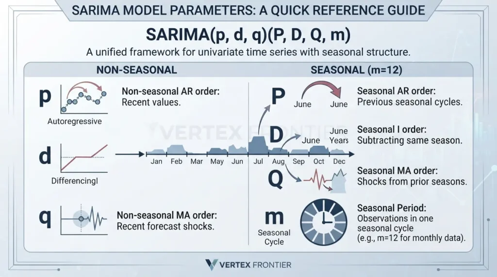
The standard notation is:
SARIMA(p, d, q)(P, D, Q, m)The current statsmodels SARIMAX API names the final seasonal argument s, while many forecasting texts use m. They refer to the same idea: the number of observations in one seasonal cycle.
SARIMA parameters at a glance
| Term | Meaning | Practical question |
|---|---|---|
| p | Non-seasonal autoregressive order | How many recent values may carry useful information? |
| d | Non-seasonal differencing order | How much trend-related non-stationarity should be removed? |
| q | Non-seasonal moving-average order | How can recent forecast shocks affect the next values? |
| P | Seasonal autoregressive order | How many previous seasonal cycles may matter? |
| D | Seasonal differencing order | Should the same season in the previous cycle be subtracted? |
| Q | Seasonal moving-average order | Can shocks from prior seasonal cycles improve the forecast? |
| m | Length of one seasonal cycle | What does “same season” mean in this dataset? |
ARIMA versus SARIMA: what changes?
ARIMA is not useless when a series is seasonal. The more precise statement is that a non-seasonal ARIMA specification does not explicitly include seasonal operators. You can seasonally adjust data first, include selected long lags, or use another model, but those are different modeling decisions.
SARIMA expresses the seasonal structure directly. That usually makes the model easier to reason about than adding dozens or hundreds of ordinary lags. Still, a seasonal pattern is not enough reason to use SARIMA automatically. A seasonal-naive benchmark may already capture most of the predictable pattern, and a model with external drivers may be more appropriate when promotions, weather, holidays, or prices explain the changes.
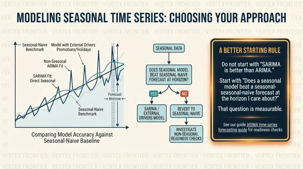
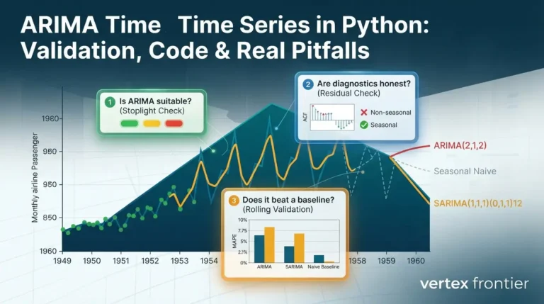
For the non-seasonal readiness checks, see our guide ARIMA time-series forecasting guide. This article concentrates on the seasonal decisions that should come after those checks.
Choose the seasonal period m before the other orders
The seasonal period is not the number of rows in your dataset. It is the number of observations in one repeating cycle.
| Data frequency | Possible seasonal cycle | Typical `m` |
|---|---|---|
| Monthly | Yearly | 12 |
| Quarterly | Yearly | 4 |
| Daily | Weekly | 7 |
| Hourly | Daily | 24 |
| Weekly | Yearly | 52 approximately |
These are starting points, not guarantees. Daily data may contain weekly, yearly, and holiday effects at the same time. The basic seasonal_order argument represents one seasonal period. If two seasonal cycles are important, consider a model designed for multiple seasonality, such as dynamic harmonic regression with Fourier terms, or another method appropriate to the data.
Stationarity: transform first, difference only as needed
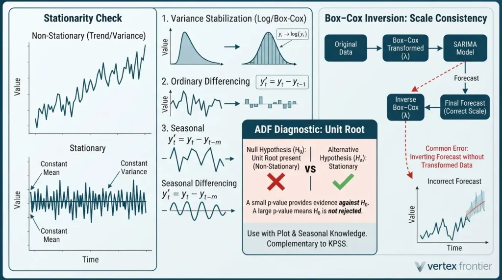
Forecasting references describe a stationary series as one whose statistical properties do not depend on when it is observed. In practice, you inspect its level, variance, autocorrelation, and seasonal behavior rather than relying on one test result.
Three operations are easy to confuse:
- A variance-stabilizing transformation such as log or Box–Cox changes the scale of the observations.
- Ordinary differencing subtracts the previous observation:
y[t] - y[t-1]. - Seasonal differencing subtracts the observation from the previous cycle:
y[t] - y[t-m].
The Forecasting: Principles and Practice ARIMA chapter explains that ordinary and seasonal differences can both be needed, but differencing is not an automatic “the more, the better” operation. Over-differencing can create unnecessary noise and make the model harder to fit.
ADF is a diagnostic, not a pass/fail button
The null hypothesis of the statsmodels Augmented Dickey–Fuller test is that the series contains a unit root. A small p-value provides evidence against that null under the selected regression specification. A large p-value means you did not reject the unit-root null; it does not prove that the series is non-stationary.
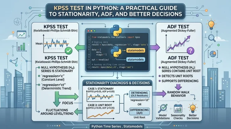
Use ADF with a plot, seasonal knowledge, and when helpful, the complementary KPSS perspective. Vertex Frontier’s KPSS guide explains why “fail to reject” is the correct wording when a test does not provide enough evidence against stationarity.
Box–Cox: the scale must remain consistent
SciPy’s Box–Cox documentation requires positive input when estimating lambda. If the model is fitted to Box–Cox-transformed data, the forecast must be inverted with the same lambda using SciPy’s inverse Box–Cox function.
That detail matters. A common tutorial error is to transform one column, fit SARIMA to the original column, and then inverse-transform the forecast. The code may execute, but the forecast is no longer on a coherent scale.
A reproducible SARIMA workflow in Python
The code below assumes a CSV named airline-passengers.csv with two columns: Month and Passengers. It uses a chronological split, estimates the Box–Cox lambda on training data only, fits SARIMA on the transformed training series, returns prediction intervals, and converts the forecast back to the original scale.
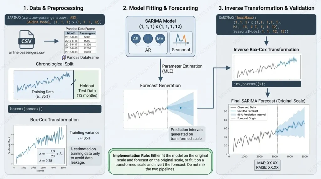
The example is deliberately conservative. It does not claim that one fixed order is correct for every dataset.
Python:
from __future__ import annotations

import numpy as np
import pandas as pd
import matplotlib.pyplot as plt

from scipy.special import inv_boxcox
from scipy.stats import boxcox
from sklearn.metrics import mean_absolute_error, root_mean_squared_error
from statsmodels.tsa.statespace.sarimax import SARIMAX

# Load and validate the time series.
df = pd.read_csv("airline-passengers.csv", parse_dates=["Month"])
df = (
    df.sort_values("Month")
      .set_index("Month")
      .asfreq("MS")
)

if df["Passengers"].isna().any():
    raise ValueError("Fill or investigate missing monthly observations first.")

series = df["Passengers"].astype(float)

# Keep the final seasonal cycle for an untouched holdout.
horizon = 12
train = series.iloc[:-horizon]
test = series.iloc[-horizon:]

# Box-Cox requires strictly positive values.
if (train <= 0).any():
    raise ValueError("Box-Cox requires positive training values; use another transformation or a justified shift.")

train_bc, lambda_ = boxcox(train.to_numpy())
train_bc = pd.Series(train_bc, index=train.index, name="Passengers_boxcox")

# Candidate chosen as a starting point, not as a universal answer.
model = SARIMAX(
    train_bc,
    order=(1, 1, 1),
    seasonal_order=(1, 1, 1, 12),
    trend="n",
    enforce_stationarity=True,
    enforce_invertibility=True,
)
results = model.fit(disp=False)

# get_forecast provides a forecast object with intervals.
forecast_result = results.get_forecast(steps=len(test))
forecast_frame = forecast_result.summary_frame(alpha=0.05)

forecast = inv_boxcox(forecast_frame["mean"].to_numpy(), lambda_)
lower = inv_boxcox(forecast_frame["mean_ci_lower"].to_numpy(), lambda_)
upper = inv_boxcox(forecast_frame["mean_ci_upper"].to_numpy(), lambda_)

forecast = pd.Series(forecast, index=test.index, name="SARIMA")
lower = pd.Series(lower, index=test.index, name="lower_95")
upper = pd.Series(upper, index=test.index, name="upper_95")

mae = mean_absolute_error(test, forecast)
rmse = root_mean_squared_error(test, forecast)
print(f"MAE: {mae:.2f}")
print(f"RMSE: {rmse:.2f}")
print(results.summary())

ax = series.plot(figsize=(12, 5), label="Observed", color="#1f2937")
forecast.plot(ax=ax, label="SARIMA forecast", color="#4169e1")
ax.fill_between(test.index, lower, upper, color="#4169e1", alpha=0.16, label="95% interval")
ax.axvline(test.index[0], color="#9ca3af", linestyle="--", label="Forecast origin")
ax.set_title("SARIMA forecast with prediction interval")
ax.legend()
plt.tight_layout()
plt.show()
trend="n" is an explicit choice here because the integrated model already handles differencing and the example is meant to keep the seasonal structure visible. Trend and intercept choices should be tested rather than copied blindly. The statsmodels SARIMAX documentation documents the available trend options and their defaults.
The interval code above is intentionally simple: it back-transforms the reported bounds. For strongly nonlinear transformations, interval interpretation on the original scale deserves extra care, so treat the result as a model output to validate rather than a guarantee of calibrated coverage.
How to choose p, d, q, P, D, Q, and m
ACF and PACF are useful because they show how a series relates to its own past. But the familiar shortcut, “PACF gives p, ACF gives q”—works most cleanly for simple pure AR or pure MA processes. In a mixed ARMA or seasonal model, both plots can tail off, overlap, or become difficult to interpret.
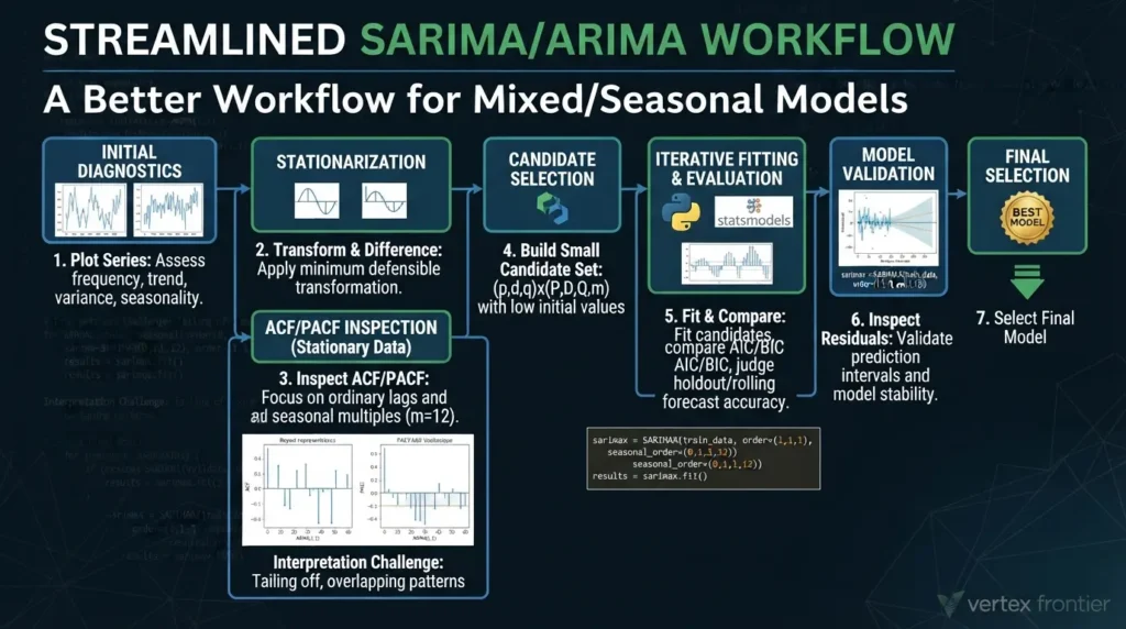
A better workflow is:
- Plot the original series and identify its frequency, trend, variance changes, and possible seasonal cycles.
- Choose
mfrom the data frequency and domain knowledge. - Apply the minimum defensible transformation and differencing.
- Inspect ACF and PACF of the resulting series. Look first at ordinary lags and then at multiples of
m. - Build a small candidate set, usually with low values such as 0 or 1 for seasonal orders unless evidence supports more.
- Fit each candidate on the same training data.
- Compare AIC or BIC among comparable fits, then judge forecast accuracy on rolling or holdout forecasts.
- Inspect residuals and prediction interval behavior before selecting the final model.
Berkeley’s ARIMA and SARIMA lecture shows why ACF/PACF identification becomes difficult for mixed ARMA processes and why seasonal lags should be interpreted as patterns, not automatic instructions.
A small grid search can help organize candidates, but it should not replace reasoning:
Python:
from itertools import product

candidates = []
for order in product([0, 1, 2], repeat=3):
    p, d, q = order
    if d not in {0, 1}:
        continue
    for seasonal in product([0, 1], repeat=3):
        P, D, Q = seasonal
        try:
            fitted = SARIMAX(
                train_bc,
                order=(p, d, q),
                seasonal_order=(P, D, Q, 12),
                trend="n",
                enforce_stationarity=True,
                enforce_invertibility=True,
            ).fit(disp=False)
            candidates.append({
                "order": (p, d, q),
                "seasonal_order": (P, D, Q, 12),
                "aic": fitted.aic,
                "bic": fitted.bic,
            })
        except Exception:
            # A failed candidate is information, not a reason to hide the failure.
            continue

ranking = pd.DataFrame(candidates).sort_values("aic")
print(ranking.head(10))
This ranks in-sample likelihood criteria. It does not prove that the first row will forecast best. Use the ranked candidates in a time-based validation loop and retain the model that performs well under the real forecasting horizon.
Evaluate SARIMA against a seasonal-naive baseline
A seasonal-naive forecast sets each future observation equal to the most recent observation from the same season. For monthly data, next February starts from the latest February; for quarterly data, next Q2 starts from the latest Q2. The forecasting toolbox treats seasonal-naive forecasts as an important benchmark for seasonal series.
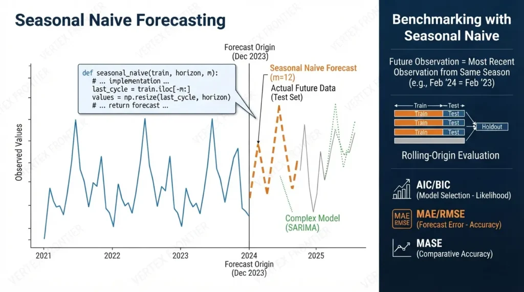
Python:
def seasonal_naive(train: pd.Series, horizon: int, m: int) -> pd.Series:
    if len(train) < m:
        raise ValueError("Need at least one complete seasonal cycle.")
    last_cycle = train.iloc[-m:].to_numpy()
    values = np.resize(last_cycle, horizon)
    index = pd.date_range(
        start=train.index[-1] + (train.index[1] - train.index[0]),
        periods=horizon,
        freq=train.index.freq,
    )
    return pd.Series(values, index=index, name="seasonal_naive")

baseline = seasonal_naive(train, horizon=len(test), m=12)
print("Seasonal-naive MAE:", mean_absolute_error(test, baseline))
print("SARIMA MAE:", mean_absolute_error(test, forecast))
For a real project, use rolling-origin evaluation instead of relying on one holdout. Train at several historical forecast origins, predict the same operational horizon, and average the errors. That approach is slower, but it tests whether the apparent advantage survives across time rather than depending on one lucky split.
Do not confuse model-selection metrics with forecast metrics:
- AIC and BIC help compare likelihood-based fits on comparable data and specifications.
- MAE and RMSE measure forecast error on the original scale.
- MASE can make errors easier to compare across series with different units.
- Prediction interval coverage checks whether the uncertainty bands are as reliable as they look.
A model with the lowest AIC is not automatically the model with the lowest future error.
Diagnose the residuals before trusting the forecast
A good residual series should not leave an obvious predictable pattern behind. The statsmodels plot_diagnostics() documentation describes a four-panel diagnostic view: standardized residuals over time, a histogram with a normal reference density, a Q-Q plot, and a residual correlogram.
Python:
import matplotlib.pyplot as plt

results.plot_diagnostics(figsize=(12, 8), lags=24)
plt.tight_layout()
plt.show()
Look for:
- residual autocorrelation at ordinary or seasonal lags;
- changing residual variance;
- clusters of unusually large errors
- a clear deviation from the assumed distribution;
- a residual mean that changes over time;
- a seasonal pattern that remains after fitting.
These diagnostics do not certify a model. A model can have visually quiet residuals and still forecast poorly.
Conversely, non-normal residuals do not automatically make every point forecast useless; they may mainly affect interval quality and inference. Use diagnostics together with out-of-sample performance.
A practical pre-publication verification gate
Before shipping a forecast or a notebook, record the following items. This turns a one-off successful run into something another analyst can reproduce and challenge.
SARIMA versus SARIMAX
SARIMAX is the statsmodels implementation name because the model can also include exogenous regressors. A pure SARIMA model is the case where no external regressor matrix is supplied.
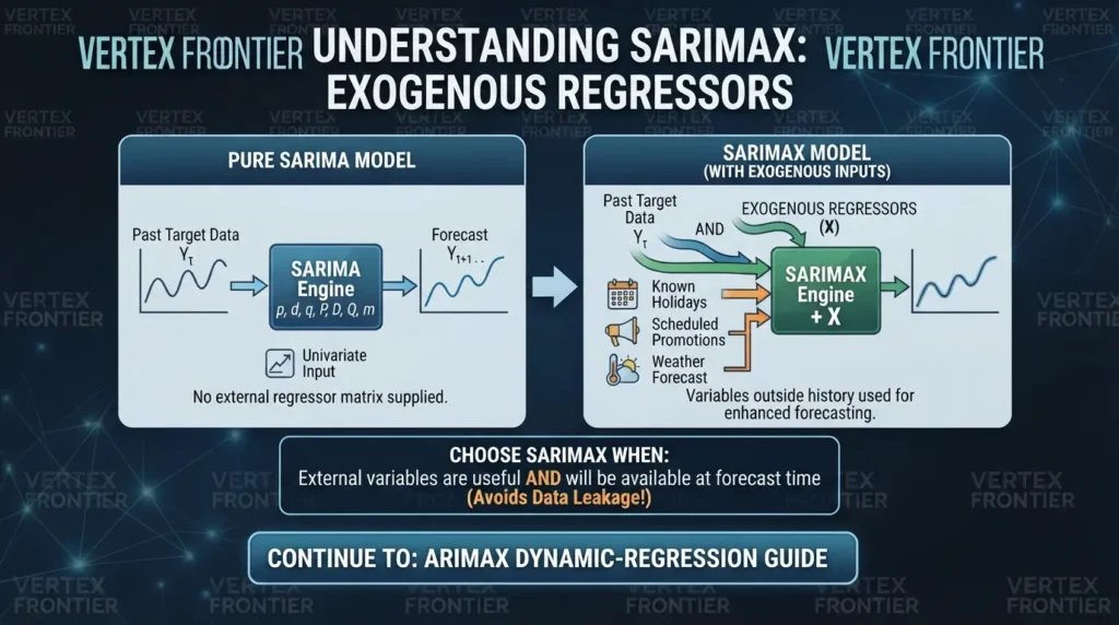
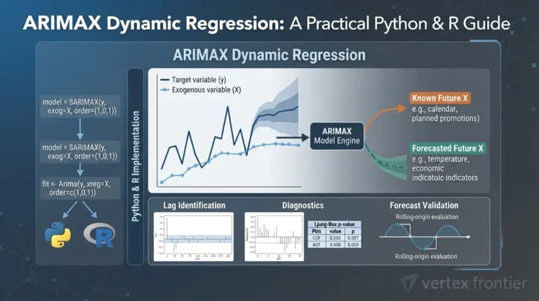
Choose SARIMAX when variables outside the target’s own history are genuinely useful and will be available at forecast time. Examples include known holiday indicators, scheduled promotions, or a separately forecast weather variable. Historical availability is not enough. If a future feature will not exist when the forecast is produced, using its observed future value creates leakage.
For the full treatment of future inputs, lagged effects, leakage, and validation, continue to our guide ARIMAX dynamic-regression guide. Keep this article focused on the seasonal univariate case and use the internal link as the handoff point.
When SARIMA is the wrong tool
SARIMA is a strong candidate when the target is a regular univariate series with a stable, meaningful seasonal cycle and enough history to observe that cycle repeatedly. It becomes less attractive when:
- the timestamps are irregular or the data contains unresolved missing periods;
- the series has multiple important seasonalities;
- a structural break changed the data-generating process;
- the target is intermittent with many zero values;
- the seasonal period changes over time;
- external variables explain most of the variation and are available for forecasting;
- the forecast horizon is long enough that uncertainty dominates the seasonal memory;
- a simple seasonal-naive model performs as well or better.
This is not a failure of classical forecasting. It is a model-boundary decision. The best forecast is the model that wins under the information available at the moment the forecast is made.
Common SARIMA mistakes
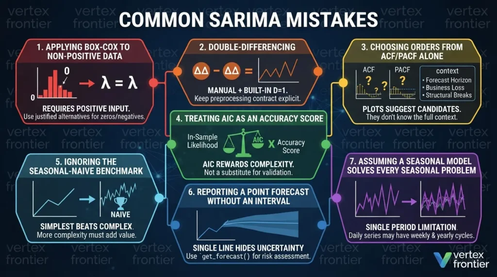
1. Applying Box–Cox to non-positive data
SciPy’s Box–Cox implementation requires positive input when estimating lambda. Use a justified alternative for zeros and negative values; do not add an arbitrary constant without documenting what that changes.
2. Double-differencing
If the series is manually seasonally differenced and the fitted model also uses D=1, the seasonal operation may be applied twice. Keep the preprocessing contract explicit: either let SARIMAX perform the differencing or pass an already transformed series with the model orders adjusted accordingly.
3. Choosing orders from ACF/PACF alone
Plots suggest candidate structures. They do not know your forecast horizon, business loss function, missing-data process, or structural breaks.
4. Treating AIC as an accuracy score
AIC rewards in-sample likelihood with a complexity penalty. It is not a substitute for time-based validation against future observations.
5. Ignoring the seasonal-naive benchmark
If a seasonal-naive forecast is already difficult to beat, a more complicated model may add maintenance cost without adding forecast value.
6. Reporting a point forecast without an interval
A single line hides the range of plausible outcomes. Use get_forecast() when the decision depends on uncertainty, inventory risk, staffing, or capacity.
7. Assuming a seasonal model solves every seasonal problem
A daily series can contain weekly and yearly patterns. One seasonal period in a standard SARIMA specification cannot represent every cycle at once.
Final decision rule
SARIMA is worth keeping when it adds forecast skill or useful uncertainty information beyond a credible seasonal-naive baseline, under a validation design that matches the real forecasting task. Its value is not that it is classical, interpretable, or fashionable. Its value is that its seasonal assumptions are explicit, testable, and replaceable when the data proves them wrong.
That is the workflow to carry into production: define the cycle, keep the transformation pipeline honest, test a small set of candidates, compare against simple forecasts, inspect the residuals, and report uncertainty instead of hiding it.
FAQs

Was this article helpful?




[…] uses the target’s own history and error dynamics without an external predictor matrix. SARIMA adds seasonal dynamics. ARIMAX adds regressors; SARIMAX combines seasonal ARIMA errors with […]
[…] the series has a clear seasonal cycle, the seasonal extension, our guide to SARIMA forecasting, shows how to extend the same workflow without abandoning ARIMA’s […]