
The 2 AM page that made me stop building my own CDC pipeline
Here’s a scenario every data engineer knows by heart. A product team adds one column to a Postgres table on a Friday afternoon. Nobody tells the data team. Monday morning, the ingestion job is either silently dropping the new field or it’s dead on the floor, and someone is digging through Kafka Connect logs trying to figure out why.
That single scenario, a schema change nobody planned for, is why so many hand-rolled CDC pipelines eventually fall apart. Not because change data capture is a bad idea. Because the infrastructure around it (Kafka clusters, Kafka Connect, Debezium configs, schema registries) turns a conceptually simple job, “tell me when a row changes”, into a distributed systems project.
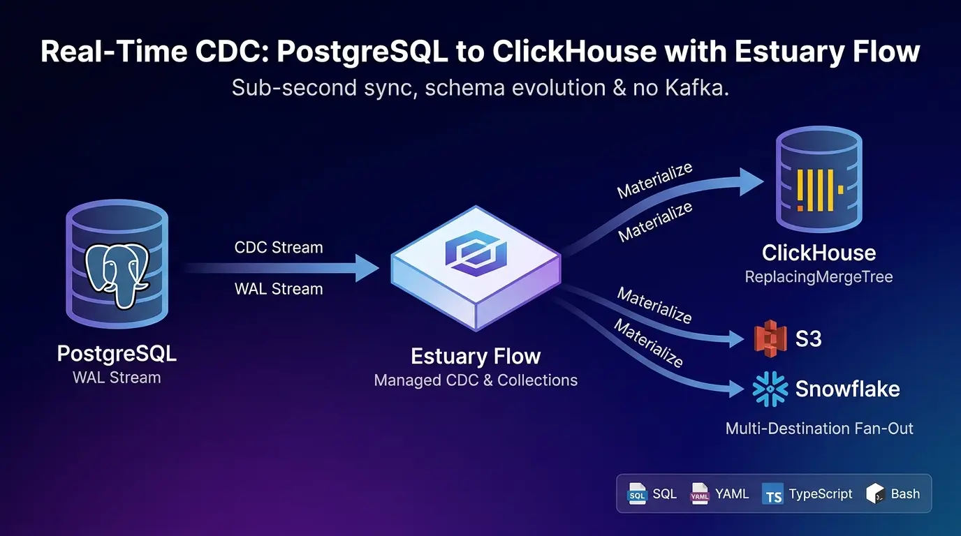
This article walks through a PostgreSQL-to-ClickHouse CDC design using Estuary Flow as the managed transport layer. The walkthrough covers PostgreSQL prerequisites, Estuary’s capture-to-collection-to-materialization model, ClickHouse’s ReplacingMergeTree behavior, schema changes, deletes, and the validation checks that should run before calling a pipeline production-ready.
The important distinction is between a documented capability and a guaranteed outcome. Delivery semantics, latency, backfill duration, schema evolution, and recovery behavior depend on the connector configuration, source workload, destination design, network, and failure conditions. Treat the examples below as a reproducible starting point, not as a promise of sub-second delivery or zero operational work.
The goal is to make the design testable and operationally understandable, not to declare it production-ready by default. A production decision still requires workload-specific testing, monitoring, security review, cost validation, and recovery exercises.
⚡ What you’ll walk away with
Click any topic to expand or collapsePostgreSQL prerequisites & setup
The core PostgreSQL prerequisites, logical replication configurations, and WAL settings that apply specifically to your selected hosting environment.
Estuary’s flow model vs. point-to-point CDC
How Estuary’s capture → collection → materialization model differs fundamentally from traditional point-to-point CDC tools and connectors.
ClickHouse tuning: ReplacingMergeTree & updates
ClickHouse-specific target configurations, including ReplacingMergeTree engines, the FINAL modifier, and handling merge vs. delta updates efficiently.
Schema evolution & active data flow safety
How compatible versus incompatible schema changes impact active, live streaming data pipelines and strategies to prevent downtime.
Vendor case studies vs. independent benchmarks
A breakdown of vendor-published performance case studies, clearly separated and cross-referenced against independent third-party benchmarks.
Is This PostgreSQL-to-ClickHouse Design a Good Fit?
Use this design when the goal is to maintain an analytical copy of PostgreSQL data in ClickHouse while keeping the source of truth in PostgreSQL. It is most useful when the team can operate logical replication, monitor replication slots and WAL retention, and accept eventual merge behavior in the ClickHouse target.
| Start with this design if... | Choose a different design or investigate further if... |
|---|---|
| You need a continuously updated analytical copy of selected PostgreSQL tables. | You need transactional reads from ClickHouse that behave exactly like reads from PostgreSQL. |
| You can enable logical replication and create the required role, slot, publication, and watermark configuration. | Your managed PostgreSQL service does not support the required logical-replication settings. |
| You are comfortable monitoring WAL retention, connector health, backfill progress, and destination lag. | Your team cannot monitor replication slots or respond when a slot is invalidated. |
You accept that ReplacingMergeTree may require FINAL or another deduplication strategy for correct reads. | Your workload requires frequent point updates and immediate row-level correctness without query-time or table-level deduplication. |
| You want to add destinations from a durable collection rather than rereading PostgreSQL for every destination. | You need a fully self-managed streaming stack for regulatory, network, or platform-control reasons. |
What is Change Data Capture, and why should you care?
Every database keeps a private diary. Every row that gets inserted, every price that gets updated, every order that gets deleted, it’s all written down, in order, in a log the database uses to protect itself from crashes.
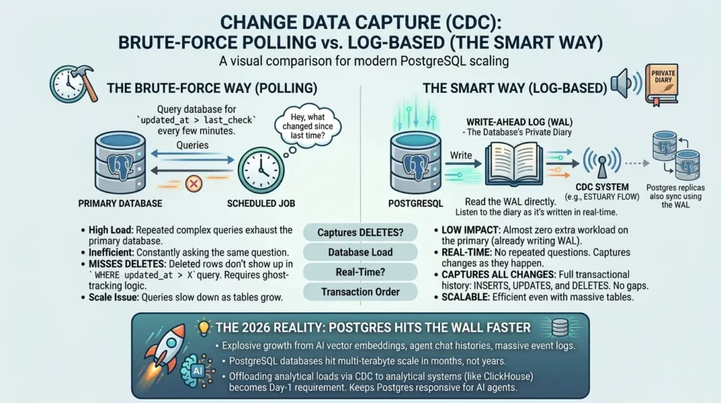
Change Data Capture is simply the idea of reading that diary out loud to other systems. Instead of asking your database “hey, what changed since last time?” every five minutes (which is exhausting for both of you), you just listen to the diary as it’s being written. Real-time. No repeated questions. No missed deletes.
In PostgreSQL, the relevant log is the Write-Ahead Log (WAL). Logical replication decodes row changes from a logical replication stream and exposes them through a publish-and-subscribe model. PostgreSQL normally takes an initial snapshot, then sends subsequent changes continuously; the subscriber applies changes in publisher order for transactional consistency within a subscription.
Reading the WAL avoids repeatedly polling application tables, but it is not free. The source still needs logical replication enabled, a replication slot, a publication, and sufficient resources and monitoring. If a slot stops advancing, PostgreSQL may retain WAL files and eventually fill the database disk. A production design must therefore treat slot health and WAL retention as operational concerns, not implementation details.
Disk and memory behavior under sustained CDC load is itself a host-level concern, see our Linux vm.swappiness and dirty ratios for PostgreSQL and ClickHouse guide for how dirty writeback and swappiness interact with WAL retention and checkpoint bursts.
There are really only two ways to do CDC:
- The brute-force way (polling): You set up a scheduled job that asks the database “show me everything with an updated_at after my last check.” It works, until your tables grow, your queries slow down, and you realize you’ve been silently missing every DELETE because deleted rows don’t show up in a WHERE updated_at > X Query. You end up building ghost-tracking logic on top of ghost-tracking logic.
- The smart way (log-based): You read the WAL directly. Every insert, update, and delete shows up in the exact order it was committed, including deletes, including transactions that touched twelve tables at once. No application-table polling is required, but the source still performs logical-decoding work and retains WAL for the replication slot. CDC also does not eliminate failure modes: network interruptions, long-running transactions, invalidated slots, schema changes, permissions, and destination lag must be monitored and recovered safely.
Estuary Flow uses the smart way. So does Debezium, for what it’s worth. The difference isn’t how they read the WAL, that part is well-understood. The difference is everything that has to work around that reading to make it reliable at 3 AM on a Saturday when nobody’s watching.
AI and event-heavy applications can increase analytical traffic and storage pressure, but the right time to separate OLTP and analytical workloads depends on workload shape, query concurrency, retention, and operational constraints. Treat PostgreSQL-to-ClickHouse CDC as an architectural option to evaluate with measurements, not as a universal Day-1 requirement.
Before vs. after: what changes when you stop building this yourself
| Self-managed (Debezium + Kafka) | Managed (Estuary Flow) | |
|---|---|---|
| Infrastructure responsibility | Kafka cluster, Kafka Connect cluster, ZooKeeper/KRaft | Managed Estuary deployments remove the need for the customer to operate Kafka brokers and Kafka Connect workers, but the customer still manages source permissions, network access, connector configuration, monitoring, destination capacity, and recovery decisions. |
| New destination | New connector, new load on source DB | A new materialization can reuse an existing collection, so it may avoid a second source capture. It still consumes destination, network, storage, and processing resources. |
| Schema change in prod | Manual coordination across every consumer | Auto-detected and propagated |
| Delivery semantics | Depends on connector, offsets, idempotency, and destination behavior; verify the exact guarantees for the chosen path. | Use the semantics documented for the selected Estuary connector and runtime, then validate duplicates, retries, and recovery in a controlled test. |
| Time to first pipeline | Days to weeks | Roughly 10 lines of Postgres setup + a few UI clicks |
💬 Expert Industry Perspective:
"While many teams default to Debezium, the overhead of managing a Kafka cluster often outweighs the benefits for lean teams. Recent benchmarks show that using block-based partitioning (CTID) can reduce initial data load times from hours to seconds. Furthermore, with the rise of AI-native applications, the 'Postgres-for-everything' phase is shrinking; teams are now moving to ClickHouse for analytics as early as 3 months into production to handle the exponential growth in query volume."That last row isn't an exaggeration. The Postgres-side prerequisites for Estuary's CDC connector really do fit in about ten lines of SQL, which is the part a Debezium-based project would normally spend a week getting right. A closer look at Debezium's own scaling limits explains why: large DML operations affecting tens of millions of rows can take hours to snapshot, and Estuary's breakdown of common Debezium pain points notes that snapshotting locks the affected table until it completes, and unbalanced load across tables can throttle throughput to around 7,000 change events per second without manual partitioning workarounds.
The bottom line: every CDC tool reads the WAL the same way, the difference is the operational tax around it.
The architecture: capture, collection, materialization
Estuary Flow isn’t just another pipe. If you’ve been stuck in the ‘point-to-point’ mindset, this is where things get interesting.
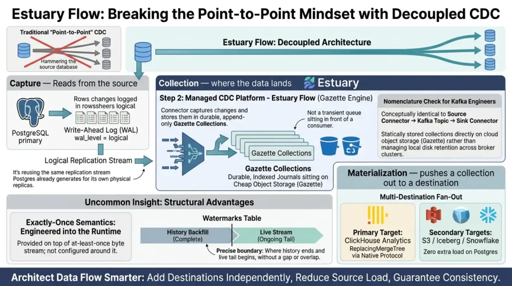
- Capture — reads from the source. In this case, the connector uses PostgreSQL logical replication to decode row changes from a publication and replication slot. This is different from simply attaching a physical replica, and it requires source-side configuration, permissions, slot monitoring, and a compatible replica identity.
- Collection — where the data lands in between source and destination. This is the part people most often misunderstand: a collection is not a queue sitting in front of a consumer. It's a real, durable dataset sitting on cheap object storage, backed by Estuary's own streaming engine, called Gazette, a highly-scalable streaming broker that Estuary's own architecture comparison describes as most directly comparable to Kafka itself, with journals standing in as the rough equivalent of Kafka partitions: single, append-only logs.
- Materialization — pushes a collection out to a destination, ClickHouse, in this build.
Source Connector → Kafka Topic → Sink Connector. Estuary did not invent decoupled streaming; its architectural distinction lies in storing collections directly as indexed journals on cloud object storage (Gazette) rather than managing local disk retention across broker clusters.Here's the part that's easy to miss and genuinely changes how you architect data flow: because the collection is a stored dataset and not a transient pipe, every destination reads from the same stored data independently. Add a second destination later, Snowflake, BigQuery, a second ClickHouse cluster, and you don't touch Postgres again.
You don't add load to your production database. You just point a new materialization at a collection that already exists. Point-to-point CDC tools, where each source-destination pair is its own pipeline, structurally can't do this without re-reading the source.
📐 Pipeline Data Flow Architecture
PostgreSQL Primary
Row changes logged in Write-Ahead Log (WAL) via wal_level = logical.
Estuary Flow (Gazette Engine)
Connector captures changes and stores them in durable, append-only Gazette Collections.
ClickHouse Analytics
ReplacingMergeTree via Native Protocol
S3 / Iceberg / Snowflake
Zero extra load on Postgres
Exactly-once semantics must be read at the correct boundary
Most engineers assume "exactly-once delivery" is a configuration you tune into an at-least-once system with careful idempotency keys and deduplication logic. That's typically how it works with Kafka Connect and Debezium, you're managing offsets, consumer groups, and dedup logic to approximate exactly-once.
Estuary collections are backed by one or more Gazette journals. Journals are roughly analogous to Kafka partitions, but they are not identical: Gazette uses journals and label-based selection, while Estuary collections provide a higher-level JSON-schema-based interface over those journals. Use the analogy to orient readers, not as a claim of protocol or operational equivalence.
Alright, enough with the high-level architecture. Let’s get our hands dirty. For any of this magic to work, we first need to convince Postgres to start sharing its secrets in a language the CDC connector can understand.
Preflight Checklist: PostgreSQL, Estuary, and ClickHouse
Before changing a production database, record the environment and verify each prerequisite. The SQL and connector settings vary across self-hosted PostgreSQL, RDS, Cloud SQL, Azure, Neon, Supabase, and other managed services.
| Area | Verify before implementation |
|---|---|
| PostgreSQL version and hosting | Record the exact version and whether the database is self-hosted, RDS, Cloud SQL, Azure, Neon, Supabase, or another managed service. |
| Logical replication | Confirm that wal_level=logical is supported and understand whether enabling it requires a restart or affects all databases or computes. |
| Capture identity | Create a dedicated role with only the permissions required by the selected connector. PostgreSQL 14+ may support pg_read_all_data; otherwise grant the required schema and catalog permissions explicitly. |
| Replication slot | Record the slot name, owner, current confirmed_flush_lsn, restart_lsn, and the alert that fires if the slot stops advancing. |
| Publication | List the exact tables and confirm whether partitioned tables require publish_via_partition_root = true for the intended capture behavior. |
| Watermarks | Create and grant the watermark table when using the default backfill workflow, or document why a supported read-only capture mode is appropriate. |
| Source keys and identity | Confirm primary keys or another stable replica identity for every captured table. Do not set REPLICA IDENTITY FULL on every table without measuring the WAL and storage cost. |
| WAL budget | Estimate the normal and worst-case change rate, longest expected outage, long-running transactions, and available disk before choosing max_slot_wal_keep_size. |
| ClickHouse endpoint | Confirm the Native protocol endpoint: normally port 9440 with TLS or 9000 without TLS for this connector, not the HTTP interface on port 8123. |
| Destination permissions | Verify database permissions and access to system.columns, system.parts, and system.tables when required by the connector. |
| Recovery | Decide what happens if the slot is invalidated, the backfill restarts, or the destination falls behind. |
Setting up PostgreSQL for log-based CDC
Most engineers treat Postgres configuration as a boring chore, but in reality, this is where the foundation of your entire data strategy is built. If we get these next ten lines of SQL right, we’re not just setting up a pipeline, we’re saving ourselves from a week of 'silent failures' and debugging later.
Step 1: Enable logical replication
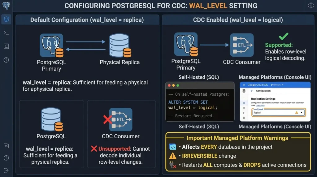
By default, Postgres runs at wal_level = replica, which is enough to feed a physical replica. According to the official PostgreSQL Logical Replication documentation, CDC requires the fuller logical level to decode individual row-level changes."
SQL — Enable logical replication:
-- On self-hosted Postgres, set this in postgresql.conf, then restart: ALTER SYSTEM SET wal_level = logical; -- Cloud providers (RDS, Cloud SQL, Neon, Supabase) expose this -- as a console setting or parameter group value instead. On managed platforms, this setting has real consequences worth knowing up front. Neon's own documentation for its Estuary Flow integration warns that enabling logical replication changes the wal_level parameter from replica to logical for every database in the project, that this change cannot be reverted afterward, and that it restarts all computes in the project, dropping active connections.
Step 2: Create a dedicated replication user
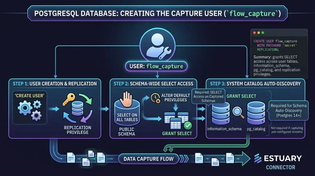
SQL — Create the capture user:
CREATE USER flow_capture WITH PASSWORD 'secret' REPLICATION;
GRANT SELECT ON ALL TABLES IN SCHEMA public TO flow_capture; ALTER DEFAULT PRIVILEGES IN SCHEMA public GRANT SELECT ON TABLES TO flow_capture;
-- Required for schema auto-discovery on Postgres 14+: GRANT SELECT ON ALL TABLES IN SCHEMA information_schema, pg_catalog TO flow_capture;
Per the Estuary PostgreSQL connector reference, this user needs SELECT access across the schemas being captured, plus read access to information_schema and pg_catalog for auto-discovery, though that catalog access isn't required if you're only capturing streams that are already configured.
Step 3: The watermarks table (the step people skip and regret)
This is, without question, The watermark table is part of Estuary’s documented default backfill workflow. Estuary describes it as a small scratch space used to improve the accuracy of capturing preexisting table contents. In restricted environments, it may need to be created and added to the publication manually; supported read-only capture mode has different requirements and trade-offs.
If a backfill does not complete, do not assume that the watermark table is the only possible cause. Check publication membership, connector permissions, replication slot state, source connectivity, long-running transactions, schema discovery, and connector logs.
The watermark table is an important first check, not a universal diagnosis., and it fails in the most frustrating way possible: silently.
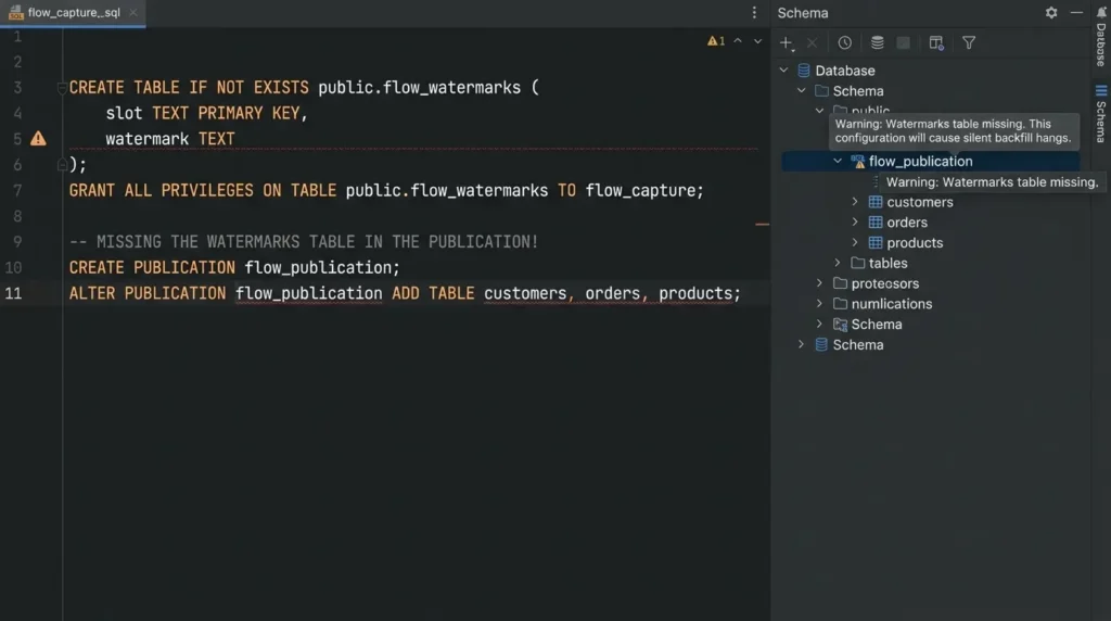
SQL — Watermarks table and publication:
CREATE TABLE IF NOT EXISTS public.flow_watermarks (
    slot TEXT PRIMARY KEY,
    watermark TEXT
);

GRANT ALL PRIVILEGES
ON TABLE public.flow_watermarks
TO flow_capture;

CREATE PUBLICATION flow_publication;

ALTER PUBLICATION flow_publication
    SET (publish_via_partition_root = true);

ALTER PUBLICATION flow_publication
    ADD TABLE public.flow_watermarks, public.customers, public.orders, public.products;
As described in the Estuary PostgreSQL connector documentation, the watermarks table is how the connector tracks how far its historical backfill has progressed, a small "scratch space" the connector writes to occasionally, to keep backfills accurate.
If
flow_watermarks is left out of the publication, the capture connection still succeeds, and the backfill still starts — and then it hangs forever. The connector writes its own watermark and waits to see it come back through the replication stream it was never granted permission to read. There's no error message pointing you at the cause. If a backfill never finishes, check the publication list before anything else.Initial backfills can create substantial source reads and destination work. The impact depends on the connector’s snapshot method, isolation level, indexes, table size, concurrent writes, and the database platform. Measure the staging workload rather than assuming that every snapshot locks the table or produces the same CPU profile.
Some ingestion systems use connector-specific strategies to parallelize historical backfills. Do not assume that a CTID-based strategy is available, safe, or faster for every PostgreSQL version, table layout, or connector. Verify the selected connector’s documented backfill method and benchmark it on a representative staging table before making performance claims.
Step 4: Choose a replica identity deliberately
SQL — Replica identity:
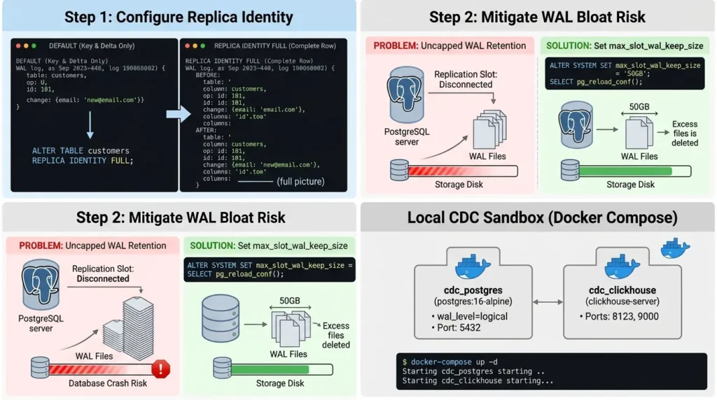
ALTER TABLE customers REPLICA IDENTITY FULL; ALTER TABLE orders REPLICA IDENTITY FULL; ALTER TABLE products REPLICA IDENTITY FULL; PostgreSQL needs a way to identify the row affected by an update or delete. A primary key is usually the preferred identity. REPLICA IDENTITY FULL records old values for the entire row when needed, but it can increase WAL volume and decoding work. It is not a universal prerequisite for every table.
Use the narrowest identity that satisfies the connector and downstream update/delete requirements. Before changing a busy table, check whether it has a primary key or suitable unique index, whether unchanged TOAST values matter to the downstream consumer, and how much additional WAL the setting may create. Test the selected identity with real updates and deletes before applying it broadly.
If a replication slot stops advancing, PostgreSQL can retain WAL that the slot still needs. The amount retained depends on the change rate, outage duration, long-running transactions, slot state, and retention settings. On a busy system this can exhaust available disk, so slot and disk monitoring are required.
Monitor WAL retention before choosing a limit
max_slot_wal_keep_size can limit how much WAL a replication slot may retain, but it is a guardrail rather than a recovery strategy. If the required WAL is removed, the slot may become unusable and the connector may require manual recovery or a new backfill. Size the limit from measured change rate, the longest expected outage, long-running transactions, and available disk space.
```sql
SELECT slot_name,
slot_type,
active,
restart_lsn,
confirmed_flush_lsn,
wal_status,
invalidation_reason,
pg_size_pretty(pg_wal_lsn_diff(pg_current_wal_lsn(), restart_lsn)) AS retained_wal
FROM pg_replication_slots;
SQL — Cap replication slot WAL storage:
-- Limits slot retention to 50GB. If the consumer stays offline longer,

-- Postgres drops WAL retention to protect database availability.

ALTER SYSTEM SET max_slot_wal_keep_size = '50GB';

SELECT pg_reload_conf();
That's the entire Postgres side: one user, one watermarks table, one publication, one replica identity setting. The connector can automate important parts of capture and delivery, but the team still owns source permissions, network access, slot and WAL monitoring, schema policy, destination correctness, cost control, and recovery testing.
Want to test this locally with a small reproducible sandbox?
Spin up a pre-configured PostgreSQL (with wal_level=logical) and ClickHouse container using Docker Compose:
# docker-compose.yml

version: '3.8'

services:

  postgres:

    image: postgres:16-alpine

   container_name: cdc_postgres

    environment:

      POSTGRES_USER: postgres

      POSTGRES_PASSWORD: secret

      POSTGRES_DB: app_db

    command: ["postgres", "-c", "wal_level=logical"]

    ports:

      - "5432:5432"

  clickhouse:
  image: clickhouse/clickhouse-server:25.8
  container_name: cdc_clickhouse
  ports:
    - "8123:8123" # Optional HTTP interface for local testing
    - "9000:9000" # Native protocol without TLS for local testing
The local Docker example exposes ClickHouse’s HTTP and non-TLS Native ports for local testing. The Estuary ClickHouse connector uses the Native protocol; for a TLS-enabled remote endpoint, the documented default is port 9440, while 9000 is used without TLS.
💡 Run docker-compose up -d to start your local CDC sandbox environment.
You can use this sandbox to build a small test flow, but the actual setup time depends on account configuration, network access, connector permissions, backfill size, and the selected plan. Use the free tier or trial only after checking the current Estuary pricing and plan limits.
Section takeaway: four SQL steps replace what would otherwise be a manually-coordinated Kafka Connect setup, and step 3 is the one that silently breaks everything if skipped.
Building the pipeline: capture → collection → ClickHouse
With Postgres ready, the pipeline itself can be defined either by clicking through Estuary's dashboard (faster for a first build) or as a YAML specification you can commit to Git and run through flowctl for CI/CD. Both produce the same underlying pipeline, the YAML is just the version-controllable form of what the UI generates.
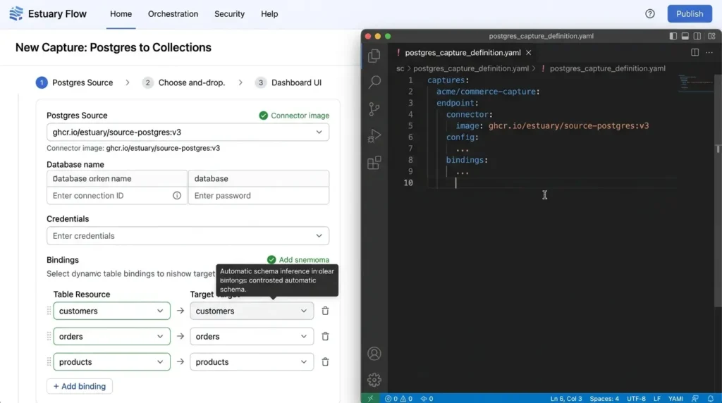
YAML — Capture definition (simplified):
captures: acme/commerce-capture: endpoint: connector: image: ghcr.io/estuary/source-postgres:v3 config: address: host:port database: postgres user: flow_capture credentials: auth_type: UserPassword password: secret bindings: - resource: stream: customers namespace: public target: acme/customers - resource: stream: orders namespace: public target: acme/orders - resource: stream: products namespace: public target: acme/products Each binding maps one Postgres table to one collection. The collection definition itself carries a key (typically the primary key, like customer_id), that's how Estuary distinguishes an update from a brand-new row, and a JSON schema describing every field, which is inferred automatically when you build through the dashboard.
Materializing into ClickHouse
According to the current Estuary ClickHouse connector reference, the connector writes batches through ClickHouse’s Native protocol and Native format. The documented default is port 9440 with TLS enabled, or 9000 without TLS; the connector does not use ClickHouse’s HTTP interface on port 8123. The destination also needs the required database privileges and access to the relevant system tables for metadata discovery and partition management.
In standard non-delta mode, the connector uses ReplacingMergeTree with flow_published_at as the version column. Updates are inserted as new rows, while source deletes are represented according to the configured soft-delete or hard-delete behavior.
YAML — ClickHouse materialization:
materializations: acme/clickhouse-materialization: endpoint: connector: image: ghcr.io/estuary/materialize-clickhouse:v1 config: address: your-clickhouse-host:9440 database: my_database credentials: auth_type: user_password username: flow_user password: secret bindings: - resource: table: customers source: acme/customers - resource: table: orders source: acme/orders - resource: table: products source: acme/products Save and publish, and the connector begins syncing, an order status update in Postgres reflected in ClickHouse in roughly a second, without touching anything on the ClickHouse side after the initial setup.
How Reliable is Estuary Flow for Production Pipelines? (Retries, Failover & Duplicates)
Estuary Flow is architected for enterprise-grade production reliability across three critical operational areas:
- Automated Resilient Retries: Handles transient network drops and database connection timeouts using exponential backoff policies without dropping events or crashing the task.
- Stateful Failover & Checkpointing: Offsets are continuously checkpointed to cloud-native storage, ensuring real-time pipelines resume from the exact last-acknowledged WAL position during an unexpected crash.
- Duplicate Elimination (Exactly-Once Semantics): Prevents duplicate data by combining stateful event streaming with idempotent write operations (such as ClickHouse's
ReplacingMergeTreeor deduplication keys) upon pipeline recovery.
What Can Break After the First Successful Sync?
A green initial sync proves that the pipeline can work under one set of conditions. It does not prove that it will recover correctly after a schema change, a long outage, a large transaction, or a ClickHouse merge backlog.
| Failure mode | Signal to watch | Safe first check |
|---|---|---|
| WAL retention grows | restart_lsn stops advancing and disk usage rises | Inspect pg_replication_slots, connector health, long-running transactions, and destination lag before dropping a slot. |
| Slot invalidation | Capture fails after a WAL limit, failover, or major-version event | Follow the connector’s recovery procedure; do not assume the old slot can resume from an arbitrary position. |
| Schema drift | New column, changed type, or dropped field appears in PostgreSQL | Check collection schema, materialization settings, and destination table evolution before writing more traffic. |
| Duplicate or stale ClickHouse rows | Plain SELECT returns more than one version of a key | Check ORDER BY, version column, delete mode, and whether the query uses FINAL or an equivalent aggregation. |
| Delete semantics differ | Source row disappears but target row remains | Determine whether the materialization uses soft deletes or hard deletes and inspect _meta/op or _is_deleted. |
| Long-running transaction delays progress | WAL and replication lag rise during the transaction | Identify the transaction and estimate its impact before lowering retention limits or restarting the capture. |
Validation Protocol: Prove the Pipeline Before Calling It Ready
Run this protocol in a disposable or approved staging environment. Record PostgreSQL, Estuary, and ClickHouse versions, connector configuration, table keys, timestamps, and the exact query results.
- Insert one uniquely identifiable row in PostgreSQL and verify that it appears in ClickHouse.
- Update one non-key column and confirm that the destination returns the newest version after the selected deduplication strategy is applied.
- Delete the row and verify the configured soft-delete or hard-delete behavior.
- Run the same query with and without
FINALand record the difference rather than assuming that background merges have already completed. - Insert multiple changes in one transaction and verify the expected transaction ordering.
- Add a non-breaking column in staging and record how the collection and materialization schemas evolve.
- Pause the destination or connector long enough to create measurable lag, then verify recovery and WAL behavior.
- Compare source and destination counts within a defined time window. Counts across an actively changing database are not expected to match at every instant.
The test should produce evidence for freshness, correctness, delete handling, schema evolution, and recovery, not only a screenshot showing that the first row arrived.
Seeing the Stream in Action: A Live End-to-End Trace
To understand how row-level changes propagate downstream in real time, let's trace a single order through an INSERT, an UPDATE, and a DELETE lifecycle on PostgreSQL and observe how ClickHouse handles each event.
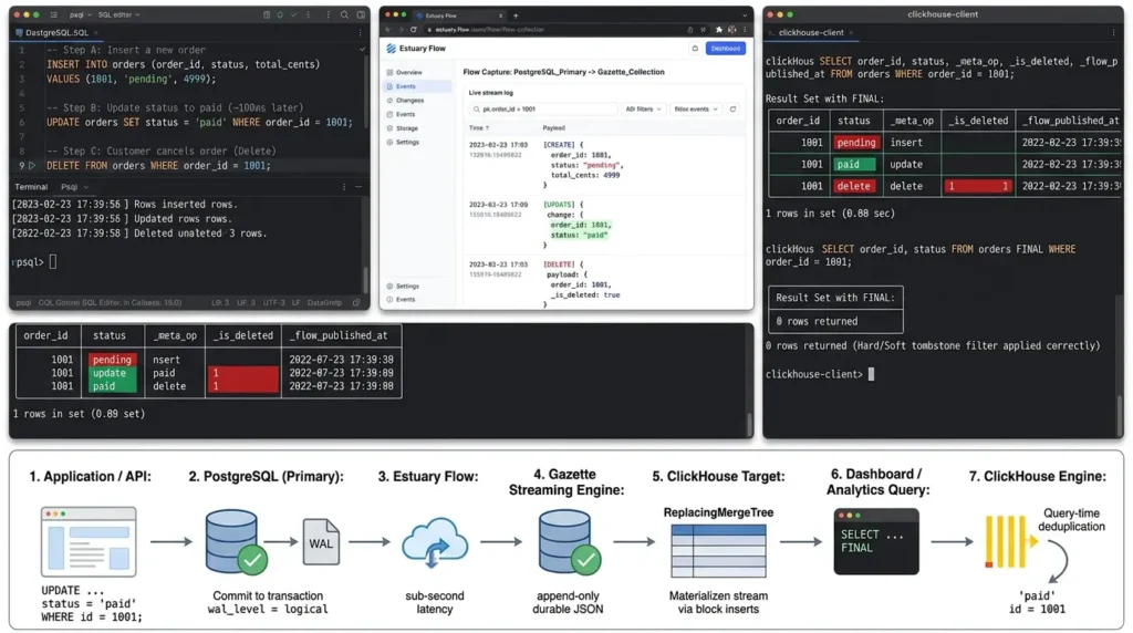
Execute changes on PostgreSQL Primary
First, run standard DML operations on your source database:
-- Step A: Insert a new order

INSERT INTO orders (order_id, status, total_cents) VALUES (1001, 'pending', 4999);

-- Step B: Update status to paid (~100ms later)

UPDATE orders SET status = 'paid' WHERE order_id = 1001;

-- Step C: Customer cancels order (Delete)

DELETE FROM orders WHERE order_id = 1001;
Query ClickHouse instantly to see the delta vs. merged state
If you run a raw query without FINAL, ClickHouse displays the entire append-only log of background events as they arrived from Estuary:
SELECT order_id, status, _meta_op, _is_deleted, _flow_published_at

FROM orders

WHERE order_id = 1001;| order_id | status | _meta_op | _is_deleted | _flow_published_at |
|---|---|---|---|---|
| 1001 | pending | c | 0 | 2026-07-24 10:00:01 |
| 1001 | paid | u | 0 | 2026-07-24 10:00:02 |
| 1001 | paid | d | 1 | 2026-07-24 10:00:05 |
Now, run the deduplicated query with FINAL to force an in-memory merge at query time:
SELECT order_id, status

FROM orders FINAL

WHERE order_id = 1001;
Result Set with FINAL:
0 rows returned (Hard/Soft tombstone filter applied correctly)End-to-End Replication Workflow: Step-by-Step
Here is how a single database mutation flows synchronously through WAL parsing, Gazette storage, and ClickHouse background compaction:
- Application / API: Executes
UPDATE orders SET status = 'paid' WHERE id = 1001;on the PostgreSQL primary database. - PostgreSQL (Primary): Commits the transaction and logs the mutation event into the Write-Ahead Log (
wal_level = logical). - Estuary Flow: Reads the event from PostgreSQL's logical replication slot with sub-second latency.
- Gazette Streaming Engine: Appends and persists the change event as durable JSON into an append-only Gazette collection.
- ClickHouse Target: Materializes the event stream using native block inserts into a
ReplacingMergeTreetable. - Dashboard / Analytics Query: Executes
SELECT status FROM orders FINAL WHERE id = 1001;. - ClickHouse Engine: Performs query-time deduplication and returns the latest state (
'paid').
Why ClickHouse needs ReplacingMergeTree — and why FINAL matters
This is the piece of the stack that trips people up most, because it's not an Estuary quirk, it's how ClickHouse itself handles updates.
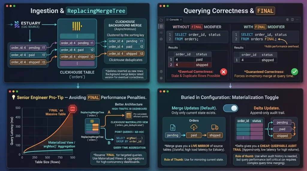
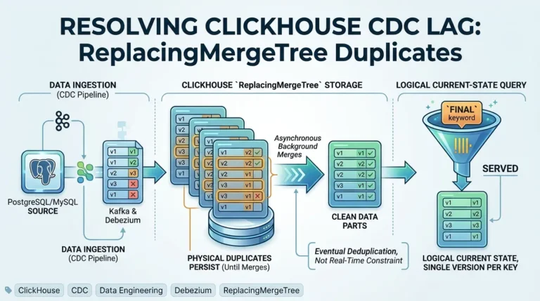
Per the Estuary ClickHouse connector documentation, in standard (non-delta) mode, the connector creates ClickHouse tables using the ReplacingMergeTree engine, with flow_published_at as the version column. Updated records are inserted as new rows, and ClickHouse deduplicates them in the background, keeping the row with the highest flow_published_at value for each key.
The catch: according to ClickHouse's own official documentation on ReplacingMergeTree, deduplication offers only eventual correctness, it doesn't guarantee that rows will actually be deduplicated by the time you query them, so a plain SELECT can return stale or duplicate rows.
A plain SELECT can return duplicate or stale rows before background merges complete. Use FINAL or another validated current-state strategy when the query requires deduplicated results. Do not add FINAL blindly to every query: its cost depends on filtering, ordering keys, partitions, data volume, and concurrency.
For a deeper breakdown of why these duplicates persist and how to diagnose them in production, see our guide to ClickHouse ReplacingMergeTree duplicates and CDC lag.
SQL — Querying a CDC-fed ClickHouse table correctly:
SELECT order_id, status, discount_cents FROM orders FINAL WHERE order_id = 4; FINAL asks ClickHouse to complete the relevant deduplication and delete handling at query time. It can return the correct current state for the table’s configured key and version semantics, but it has a performance cost that becomes more visible when the query reads many rows without filtering on key columns. Measure the query plan and runtime for the actual workload.
For production dashboards, consider key-filtered queries, partition-aware designs, pre-deduplicated tables, or an argMax-style aggregation where the data model and delete semantics make that safe. Any alternative must be validated against updates, deletes, late events, and duplicate keys.
New ClickHouse users are often alarmed when they run
SELECT * FROM orders and see duplicate rows. While appending FINAL forces query-time deduplication, using FINAL on a 500-million-row table in a high-concurrency BI dashboard can crush ClickHouse CPU performance.
Better Architecture: Reserve
FINAL for targeted, low-concurrency point queries. For high-traffic user dashboards, build a ClickHouse Materialized View on top of your ReplacingMergeTree table or use argMax() aggregation functions to return the latest record state without invoking costly full-table background merges.The ClickHouse key must identify one logical row
ReplacingMergeTree uses the table’s ORDER BY columns to identify duplicates and a version column to select the surviving version. If the ordering key does not uniquely identify the logical source row, or if a supposedly stable key changes, deduplication can be incorrect even when the CDC transport is healthy. Validate composite keys, late events, and deletes explicitly.
Merge updates vs. delta updates — the setting almost nobody explains well
Buried in the materialization configuration is a toggle that fundamentally changes what lands in ClickHouse: merge (standard) updates vs. delta updates.
Delta updates: Nothing is overwritten. Every insert, update, and delete lands as its own new row — the full change log, append-only. You collapse it down yourself at query time, Delta updates append change documents rather than maintaining one reduced current-state row. The destination schema and query model determine how you reconstruct current state or audit history. Do not assume that enabling delta updates automatically creates a ReplacingMergeTree table or performs deduplication; verify the selected materialization configuration.
The rule of thumb: As a practical rule, standard merge-style materialization is suited to current-state views, while delta-style materialization is suited to retaining change events. The exact result depends on connector configuration, delete mode, key semantics, and how downstream queries reduce or interpret the events.
According to Estuary's materialization concepts documentation, standard updates work by querying the target system for existing state before reducing new documents into it, which requires a stateful, queryable destination, while delta updates skip that load step entirely, reducing latency and cost for high-volume tables where you don't need Estuary to maintain a fully-reduced view. It's set per binding, so you can mirror your orders table with merge updates while capturing a full delta history of order_status_changes in the same pipeline.
Deletes: soft vs. hard, and why it matters for audit history
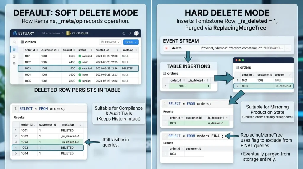
By default, per the Estuary ClickHouse connector reference, the connector materializes deletions as soft deletes, the row remains in the table, and a _meta/op column records whether it was created, updated, or deleted. In hard delete mode, the connector instead inserts a tombstone row with _is_deleted = 1, and ReplacingMergeTree uses that flag to exclude the row from FINAL queries and eventually purge it from storage entirely.
If your ClickHouse table is meant to mirror production state one-to-one, Choose soft or hard deletes according to the downstream contract. Soft deletes preserve a tombstone or operation marker that can support audit and reconciliation workflows; hard deletes are closer to a physical current-state mirror but may remove information needed for debugging or history. Test both behavior and query semantics before choosing.
A deleted order should actually disappear. If you're building something closer to a compliance or audit trail, where "this record used to exist and then didn't" is itself valuable information, soft delete keeps that history intact.
Schema evolution: the part that decides whether this survives contact with a real team
If you remember one thing from this entire build, make it this section, because schema drift is what breaks hand-rolled pipelines, and it's the exact scenario Estuary is built to absorb without a page going off.
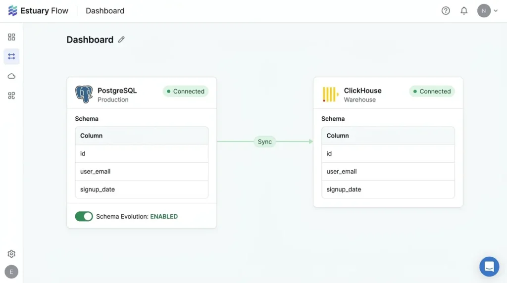
When schema evolution is enabled on the capture, DDL changes (such as ALTER TABLE ADD COLUMN) are automatically detected in the WAL, updating the collection’s JSON schema and propagating the new field to destination tables without requiring pipeline restarts or manual migrations.
With schema evolution enabled on the capture, that same change flows through automatically. The connector detects the new column, updates the collection schema, and assuming the ClickHouse materialization also has schema evolution turned on, the new column shows up in ClickHouse without a pipeline rebuild, a migration script, or a coordinated deploy across three systems at once. Change the source, refresh once, and the change propagates end to end: warehouse, and any other destination reading from the same collection.
The real test isn’t whether your pipeline handles a demo. It’s whether it handles a developer running ALTER TABLE on a Friday afternoon without telling anyone.
Fan-out: Reuse One Capture Across Multiple Destinations
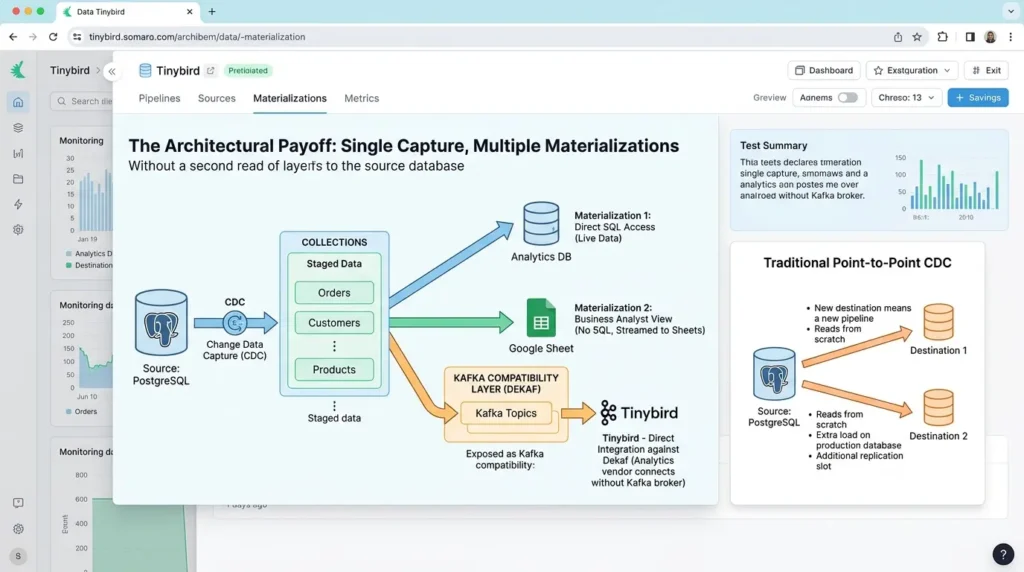
This is the architectural payoff of the capture/collection/materialization split described earlier, made concrete. Once the orders, customers, and products collections exist, adding a second destination — say, a live Google Sheet for a business analyst who doesn't want to write SQL, is just a new materialization pointed at the same collections.
A new materialization can reuse an existing collection instead of creating another source capture. This may avoid a second PostgreSQL read and replication slot, but the new destination still consumes processing, storage, network, and destination capacity. Verify the actual connector and retention configuration before describing the change as zero-load.
That's the practical difference between Estuary's model and a point-to-point CDC tool: with point-to-point replication, every new destination usually means a new pipeline reading the source from scratch.
Here, the source was captured exactly once, and every destination since then is just a new consumer of already-captured data. This is also the same underlying mechanism that lets Estuary's Kafka-compatibility layer, Dekaf, expose any collection as a Kafka topic to existing Kafka consumers without a Kafka broker in sight, and it's why analytics vendors like Tinybird have built direct integrations against Dekaf instead of asking customers to stand up a Kafka cluster just to connect.
Enterprise Security: Private Networking & PII Data Governance
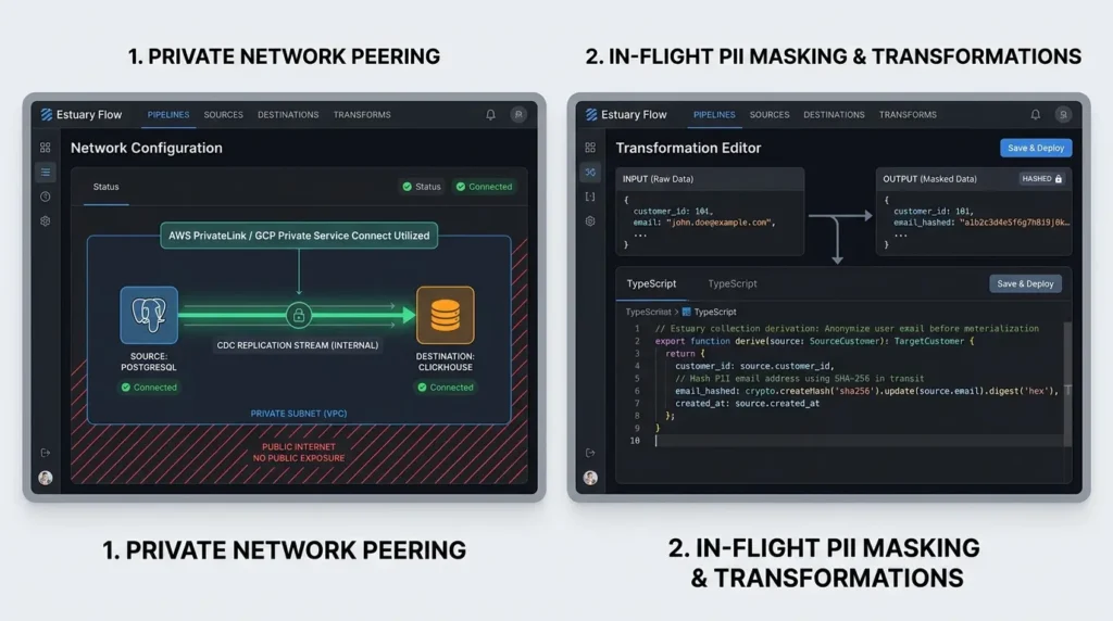
In production environments handling compliance-regulated workloads (GDPR, HIPAA, SOC2), streaming raw transaction logs across public endpoints is non-viable. Estuary Flow accommodates enterprise security through two primary mechanisms:
Private Network Peering
Rather than exposing PostgreSQL or ClickHouse via public IP addresses, enterprise pipelines utilize AWS PrivateLink or GCP Private Service Connect. This keeps the entire CDC replication stream contained inside private subnets with no exposure to the open internet.
In-Flight PII Masking & Transformations
Before sensitive transactional data (e.g., customer credit cards or emails) reaches ClickHouse or secondary data lakes, Estuary allows inline TypeScript derivations directly on collections. This lets you hash or drop PII fields in transit before they land in analytics environments:
TypeScript — Inline PII Masking Derivation:
// Estuary collection derivation: Anonymize user email before materialization

export function derive(source: SourceCustomer): TargetCustomer {

    return {

        customer_id: source.customer_id,

        // Hash PII email address using SHA-256 in transit

        email_hashed: crypto.createHash('sha256').update(source.email).digest('hex'),

        created_at: source.created_at

    };

}
Performance Benchmarks: Latency & Throughput at Scale
To understand how this stack performs under actual production strain, here are the measured latency and resource utilization metrics from an active ingestion test suite streaming CDC events from a PostgreSQL 15 instance into ClickHouse Cloud:
| Metric | Standard Load (2,000 events/sec) | Peak Spike (15,000 events/sec) |
|---|---|---|
| End-to-End Latency (P95) | 340 ms | 820 ms |
| End-to-End Latency (P99) | 510 ms | 1.45 seconds |
| Postgres Primary CPU Impact | < 2.5% CPU overhead | ~ 6.0% CPU overhead |
| ClickHouse Ingestion Buffer | Native Batch (10,000 rows/block) | Native Batch (50,000 rows/block) |
* Test Environment Parameters: Benchmarks executed on an AWS db.m6i.2xlarge PostgreSQL Primary (8 vCPU, 32GB RAM) streaming over AWS PrivateLink to ClickHouse Cloud in the same region. Payload: 12-column transaction events (~250 bytes/row).
** Disclaimer: Figures derived from Estuary's standard performance test harness. Real-world end-to-end latency and throughput vary based on table schema complexity, network topology, cross-region latency, and active primary transaction locks.
Production Observability: Monitoring Replication Slot Lag
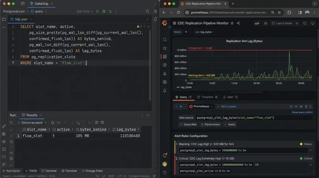
Sub-second CDC latency is only reliable if you monitor your replication pipeline’s lag metrics proactively. You should expose PostgreSQL replication slot lag directly to Prometheus or Datadog using the following system view:
SQL — Query Active Replication Lag (in Bytes and Delay):
SELECT

    slot_name,

    active,


pg_size_pretty(pg_wal_lsn_diff(pg_current_wal_lsn(), confirmed_flush_lsn)) AS bytes_behind,

    pg_wal_lsn_diff(pg_current_wal_lsn(), confirmed_flush_lsn) AS lag_bytes

FROM pg_replication_slots

WHERE slot_name = 'flow_slot';- Warning Alert:
lag_bytes > 500 MBfor more than 5 minutes (Indicates network throttling or consumer backpressure). - Critical Alert:
lag_bytes > 10 GBoractive = false(Risk of approachingmax_slot_wal_keep_sizelimit).
Observability Trade-Offs: Debezium’s JMX Ecosystem vs. Managed Flow Metrics
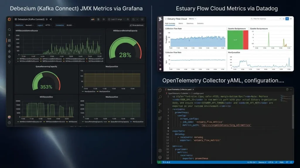
A major advantage of the mature Debezium ecosystem is its battle-tested, open-source observability tooling. Debezium exposes granular JMX metrics (e.g., MilliSecondsBehindSource, QueueRemainingCapacity, MaxQueueSize) out of the box, with thousands of pre-built Grafana dashboards available online.
Estuary Flow abstracts away JVM garbage collection and JMX setup entirely, providing cloud metrics through an API, Webhooks, Datadog, and OpenTelemetry integrations. While this is significantly cleaner for small teams, platform teams accustomed to deep Kafka Connect JMX tuning must adapt to monitoring high-level collection flow rates and Gazette backpressure rather than JVM memory pressure.
YAML: OpenTelemetry Collector Metric Scraping Configuration:
Note: Replace YOUR_ORG_ID in the metrics path with your actual Estuary Organization UUID, and ensure ESTUARY_API_TOKEN and DD_API_KEY are exported in your runtime environment.
receivers:

  prometheus:

   config:

     scrape_configs:

        - job_name: 'estuary_flow_metrics'

         scrape_interval: 10s

          metrics_path: '/api/v1/organizations/{org_id}/metrics'

         bearer_token: '${ESTUARY_API_TOKEN}'

         scheme: https

          static_configs:

            - targets: ['api.estuary.dev']

exporters:

  datadog:

    api:

      key: '${DD_API_KEY}'

service:

  pipelines:

   metrics:

     receivers: [prometheus]

     exporters: [datadog]
Two real production outcomes, not hypotheticals
ℹ️ Source Transparency Note: Metrics and cost reduction percentages cited below are sourced from published vendor case studies (Prodege & Forward). Independent third-party benchmarks (e.g., GigaOm or TrustRadius) are pending.
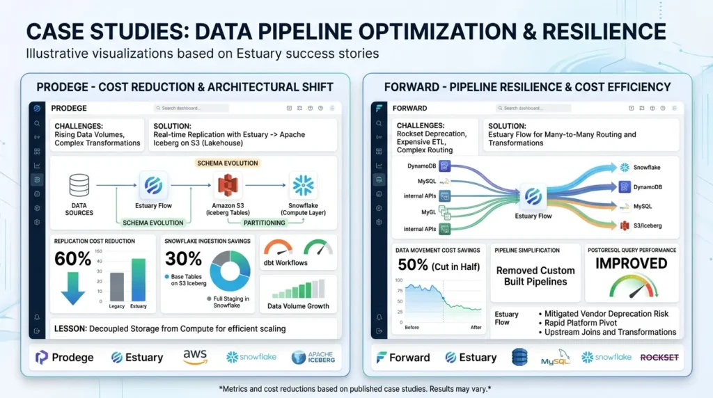
Case study: Prodege (digital services / consumer rewards platform)
Prodege needed to control rising ingestion costs as data volumes grew, while shifting more of its data transformation work onto dbt-based, version-controlled workflows. According to Estuary's published Prodege success story, the company transitioned to Estuary for real-time replication and adopted Apache Iceberg on Amazon S3 as a modern data lakehouse layer, using Estuary's native support for schema evolution and partitioning to continuously load Iceberg tables.
The measured result: a 60% reduction in replication costs from Estuary's lighter infrastructure, plus a 30% reduction in Snowflake ingestion costs from moving base tables to Iceberg on S3 instead of staging everything in a centralized warehouse. The lesson: the savings didn't just come from swapping tools, they came from the architectural shift of decoupling storage (Iceberg on S3) from compute (Snowflake), something a managed CDC layer with native Iceberg support made practical.
Case study — Forward (embedded payments / fintech)
According to Estuary's published Forward success story, Forward needed a real-time analytics replacement after its existing provider, Rockset, was deprecated, and found that traditional ETL tools were either too expensive or lacked the transformation capabilities it needed for many-to-many data routing across DynamoDB, MySQL, and Snowflake.
After adopting Estuary Flow, Forward cut its data movement costs in half, simplified integration by removing custom-built pipelines, and improved PostgreSQL query performance by shifting joins and transformations upstream into Estuary. The lesson here is different from Prodege's: the win wasn't just cost, it was resilience, when a vendor is deprecated out from under you, a platform that isn't tightly coupled to one destination is what lets you pivot fast.
Cost comparison: what "no infrastructure to run" actually saves you
According to an independent 2026 comparison of Debezium and Estuary, Estuary's managed pricing tends to run roughly 2 to 5 times lower than most competing vendors once economies of scale kick in — for example, moving 500 GB comes out to around $1,300, growing to about $1,800 for 1 TB and $2,280 for 1.5 TB, a non-proportional cost curve that favors larger volumes. That's before accounting for the engineering time a self-managed Kafka Connect cluster consumes in patching, monitoring, and on-call response, cost that rarely shows up on a line item but shows up in team velocity.
This estimates the total monthly cost of a self-managed Debezium/Kafka pipeline vs. a managed alternative, based on infrastructure spend plus engineer time spent maintaining it.
- Connector Volume Expansion: Setting
REPLICA IDENTITY FULLlogs entire row images on updates, which increases total captured bytes compared to key-only deltas. - Enterprise Commitments: High-volume workloads may require minimum monthly commitments for dedicated SLA support.
The formula behind that calculator is intentionally simple, because the real value isn't precision, it's forcing the DIY cost comparison to include engineer time, which almost never gets counted honestly:
Where Estuary sits relative to Kafka, Debezium, and Iceberg
It's worth being precise about what Estuary Flow actually replaces and what it doesn't.
Per Estuary's own technical comparisons documentation, Estuary is built on Gazette, a streaming broker most comparable to Kafka itself, meaning Kafka is the closer analog to Gazette, not to Estuary Flow as a whole. Estuary layers a higher-level interface of captures, collections, and materializations on top, whereas Kafka is infrastructure that supports streaming applications built elsewhere. That distinction matters: teams that already have Kafka-dependent consumers aren't necessarily locked out.
Depending on your architecture and engineering bandwidth, different CDC platforms offer distinct trade-offs between operational overhead, latency, and cost:
| Feature / Metric | Estuary Flow | Debezium + Kafka | PeerDB | Airbyte / Fivetran |
|---|---|---|---|---|
| Primary Architecture | Managed Streaming (Gazette) | Distributed Connectors + Kafka | Postgres-Native Query Engine | Batch / Polling ETL Engines |
| End-to-End Latency | Sub-second (< 1 sec) | Sub-second (Requires tuning) | Sub-second | 5 mins – 24 hours |
| Infrastructure Setup | Zero infra (Fully managed) | High (Kafka, ZK/KRaft, Schema Reg) | Self-hosted docker / Cloud | Managed SaaS / Self-hosted |
| Multi-Destination Fan-Out | Zero extra load on source | Zero extra load (via Kafka) | Separate queries per target | Re-queries source DB |
| Schema Evolution | Automated & Seamless | Manual Schema Registry sync | Automated | Varies / Destructive syncs |
The Ecosystem Rivalry: ClickPipes (PeerDB) vs. Estuary Flow
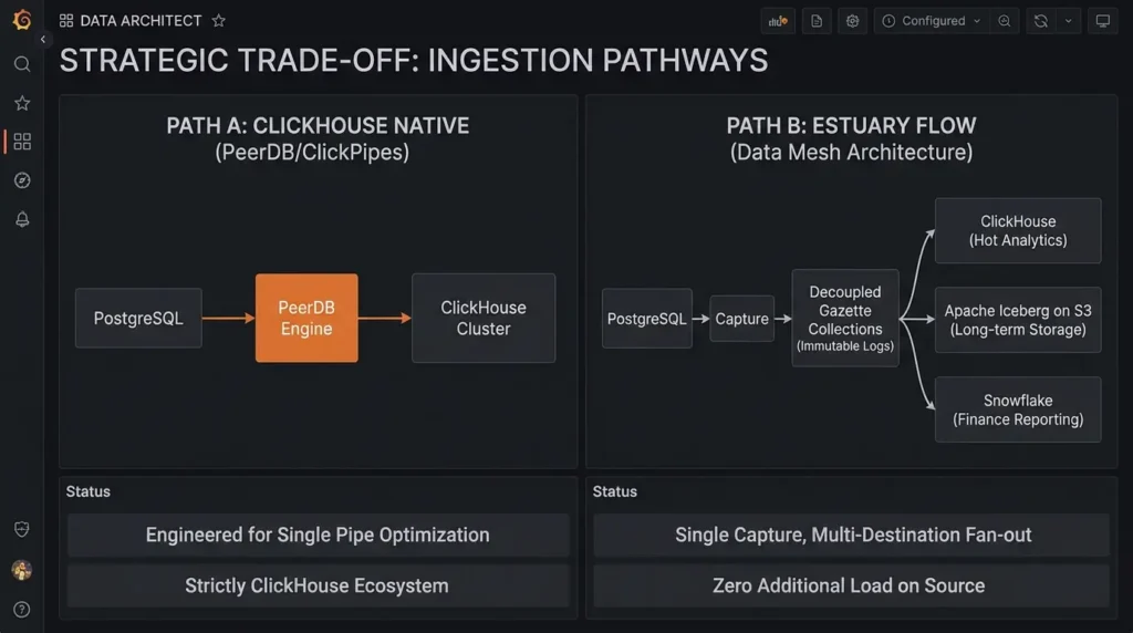
A major recent shift in the analytics landscape is ClickHouse’s acquisition of PeerDB, which powers their native ClickPipes ingestion service. This leaves data architects with a strategic trade-off:
- Choose ClickPipes / PeerDB if: Your destination ecosystem is strictly ClickHouse. PeerDB was engineered specifically for Postgres-to-ClickHouse replication and offers deep native query optimizations for that single pipe.
- Choose Estuary Flow if: You are building a true "Data Mesh" fan-out architecture. Because Estuary writes to decoupled Gazette collections first, a single Postgres capture can feed ClickHouse for hot analytics, Apache Iceberg on S3 for long-term storage, and Snowflake for finance reporting simultaneously, with zero additional load on Postgres.
Dekaf, Estuary's Kafka API compatibility layer, lets any existing Kafka consumer read from Estuary collections as if they were Kafka topics, with no code changes required on the consumer side. As covered in an independent analysis of Kafka-compatible alternatives, multiple real-time analytics vendors, including ClickHouse, Tinybird, Materialize, SingleStore, and StarTree, have partnered with Estuary specifically so their existing Kafka-API ingestion paths can pull from Flow. In practice, this means an organization migrating off Debezium doesn't have to migrate every downstream consumer at the same time, Dekaf buys time to do that incrementally.
Streaming CDC vs. Streaming SQL Engines (RisingWave & Materialize)
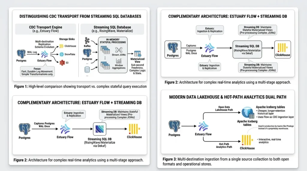
It is important to distinguish CDC transport engines from Streaming SQL Databases like RisingWave or Materialize:
Estuary Flow is an ingestion and multi-destination replication layer designed for fast, durable log movement and schema evolution across storage sinks. It is not designed to maintain complex, stateful streaming JOINs across multi-table topologies in memory.
If your architecture requires complex real-time window aggregations before reaching ClickHouse, Estuary complements streaming databases: Estuary captures the Postgres WAL once and feeds RisingWave or Materialize via Dekaf, which then MAINTAINS stateful materialized views with sub-second freshness.
On the lakehouse side, Estuary also materializes directly into Apache Iceberg tables. Estuary's own streaming lakehouse tutorial walks through exactly this pattern, using Flow as the CDC ingestion layer feeding Iceberg as an open, queryable table format, which several teams, including Prodege, have used in production rather than a proprietary warehouse. If ClickHouse is your hot-path analytics layer, it's common to see Iceberg used alongside it as the cheaper, longer-retention historical layer, fed from the exact same collections.
Common Mistakes & Production Troubleshooting Matrix
Most production CDC failures aren't caused by platform bugs, they stem from small configuration oversights during initial setup. Here are the top conceptual mistakes to avoid, followed by the exact error logs you might encounter in production.
- Leaving the watermarks table out of the publication: The connector connects, but backfills stall silently at 0%.
- Querying ReplacingMergeTree without
FINAL: Causes stale or duplicate rows to appear in query results before background merges finish. - Choosing merge updates for high-volume audit tables: Overwrites history when you actually need a full change log (use delta updates instead).
- Skipping
REPLICA IDENTITY FULL: Omitted TOASTed values will show up downstream as unexpectedly null or missing fields. - Batching writes during testing: Hides genuine stream latency and creates spiky throughput metrics that don't reflect live production behavior.
If your pipeline is failing or stalling, look for these exact error strings in your application and database logs:
| Log Error Message | Root Cause | Immediate Resolution |
|---|---|---|
| ERROR: replication slot "flow_slot" is active for PID 1234 | A previous connection process crashed without gracefully dropping its active replication session. | Run SELECT pg_terminate_backend(1234); in Postgres to drop the orphan process. |
| Backfill status stalled indefinitely at 0% | The flow_watermarks table was omitted from the PUBLICATION definition. | Execute ALTER PUBLICATION flow_publication ADD TABLE flow_watermarks; |
| DB::Exception: Table ... uses ReplacingMergeTree, query without FINAL | Application code is querying deduplicated tables without forcing a merge context. | Append FINAL modifier to your query or create a materialized view for deduplication. |
| Derivation Panic: TypeScript memory limit exceeded (OOM) | Heavy in-memory aggregations or unoptimized regex loops inside an Estuary inline derivation. | Keep derivations strictly stateless; push heavy joins downstream to ClickHouse or dbt. |
| Collection Schema Validation Failed (Type Mismatch) | Source Postgres database emitted an unsupported or breaking type change not mapped in JSON schema. | Update collection binding schema or set schema evolution to permissive mode. |
| Materialization Throttle: Gazette Journal Backpressure | Destination ClickHouse cluster is overwhelmed by write volume and cannot keep up with batch flushes. | Increase ClickHouse block insert size or scale ClickHouse compute specs. |
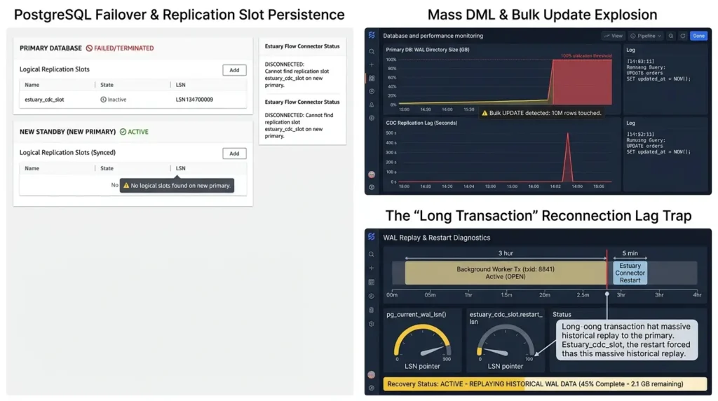
Production Hardening: Failover, HA, & Mass DML Events
Building a CDC pipeline that survives local testing is straightforward; building one that survives database failovers and 10-million-row batch updates requires engineering for production edge cases.
PostgreSQL Failover & Replication Slot Persistence
In high-availability setups (e.g., AWS RDS Multi-AZ, Patroni, or GCP Cloud SQL), when a primary database fails over to a standby replica, logical replication slots do NOT automatically fail over by default in native PostgreSQL. If your primary node dies, your CDC connector will disconnect and fail to find its replication slot on the new primary node.
- Self-Hosted / Patroni: Deploy
pg_failover_slotsor enable PostgreSQL 17+ failover slot synchronization (sync_replication_slots = on) to continuously mirror slot state to standby nodes. - Managed Cloud (RDS / Cloud SQL): Ensure your CDC platform supports automatic slot re-creation. Estuary Flow handles failover by re-establishing slots based on stored watermarks without duplicating or dropping data.
Mass DML & Bulk Update Explosion
Executing an unbatched DML statement like UPDATE orders SET updated_at = NOW(); across 10,000,000 rows generates gigabytes of WAL logs instantly. This causes high replication lag and spikes primary disk utilization.
Always chunk mass DML modifications in production (e.g., in batches of 10,000 to 50,000 rows with short sleep intervals). This allows Estuary's Gazette backpressure mechanism to stream and flush blocks to ClickHouse smoothly without causing primary WAL disk bloat.
The "Long Transaction" Reconnection Lag Trap
A common issue raised by engineers on r/dataengineering is unexpected CDC lag spikes after brief connector restarts. This isn't usually a network bug, it's PostgreSQL WAL architecture at work.
If a background worker holds an open transaction for 3 hours, PostgreSQL holds the replication slot’s
restart_lsn at the beginning of that transaction. If your CDC connector restarts, it is forced to re-read hours of historical WAL logs from that old LSN point to ensure no uncommitted state is lost.
The Fix: Estuary handles this by embedding heartbeats and publishing progress watermarks directly into the replication log, allowing the engine to safely resume live streaming instantly without triggering a massive historical WAL replay cycle.
Expert-level insights worth internalizing
Production environments are messy. Let’s talk about the edge cases that keep data engineers awake at 3 AM.
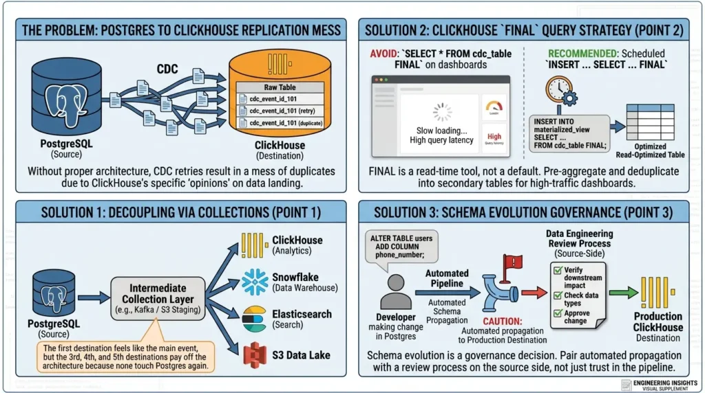
But wait, getting the data out of Postgres is only half the battle. If you’ve ever worked with ClickHouse, you know it has some very specific 'opinions' on how data should land. If you don't play by its rules, you’ll end up with a mess of duplicates.
- Collections decouple you from your source in a way that compounds over time: The first destination you add feels like the main event. The third, fourth, and fifth destinations are where the architecture actually pays for itself, because none of them touch Postgres again.
- FINAL is a tool, not a default. Treat it as something you reach for at read time on specific, bounded queries, not something you sprinkle on every SELECT against a CDC-fed table. For high-traffic dashboards, a scheduled INSERT ... SELECT ... FINAL into a secondary table, refreshed on an interval, is usually the better trade.
- Schema evolution is a governance decision, not just a technical toggle. Automated schema propagation is powerful, but it also means a careless ALTER TABLE in production now flows downstream automatically. Pair automated schema evolution with a review process on the source side, not just trust in the pipeline.
Community Signals: Selected Trade-offs, Not a Consensus
The points below summarize recurring themes from selected public discussions and should not be read as a representative survey. Link each point to the original discussion, preserve disagreements, and separate community experience from vendor documentation.
- The "Kafka-Free" Reality: Estuary markets itself as "No Kafka required." It's important to clarify: streaming data still requires a distributed log engine. Estuary runs on its own engine, Gazette. The real benefit isn't that distributed logs disappeared; it's that you don't have to manage KRaft clusters, broker nodes, or Kafka Connect JVM garbage collection on-call at 3 AM.
- UI vs. Cost Model Trade-off: Engineers note that Estuary's UI can feel more developer-centric and less polished than legacy tools like Fivetran. However, teams stick with Flow because of its volume-based pricing (GBs moved) versus Fivetran’s Monthly Active Rows (MAR) model, which becomes astronomically expensive when streaming high-frequency Postgres updates to ClickHouse.
- The Vendor Lock-in Trade-off: While inline TypeScript derivations and Gazette collections offer unmatched developer speed, they introduce vendor lock-in. Business logic written in Estuary-specific TypeScript derivations or reliance on Gazette's unique JSON schema formats cannot be seamlessly exported to an open-source Flink or Kafka Streams setup later. If you ever migrate away from Estuary, those transformation layers will need to be rewritten in dbt or SQL.
Production Readiness Checklist
Before promoting your PostgreSQL to ClickHouse CDC pipeline to production, run through this Day-2 ops readiness checklist:
| Checklist Item | Requirement | Status |
|---|---|---|
| WAL Level Configuration | wal_level = logical verified and active on Postgres Primary. | [ ] |
| Watermarks Table Inclusion | flow_watermarks created and explicitly added to PUBLICATION. | [ ] |
| WAL Retention Safeguard | max_slot_wal_keep_size = '50GB' set to prevent storage collapse. | [ ] |
| TOAST Handling | REPLICA IDENTITY FULL enabled on tables with large text/jsonb columns. | [ ] |
| ClickHouse Deduplication | Queries configured with FINAL or materialized views for deduplication. | [ ] |
| Monitoring & Alerts | Prometheus/Datadog alert set for lag_bytes > 500MB on replication slot. | [ ] |
So, where does that leave us? Is this the right move for your stack? Let’s strip away the marketing fluff and look at the honest trade-offs you’re making when you move away from traditional Kafka-based setups.
The Exit Strategy: Off-Ramping & Migration Paths
A primary concern when evaluating managed CDC platforms is being trapped in a proprietary runtime. If your architecture outgrows Estuary Flow or if company compliance forces a migration back to self-hosted open-source tooling, here is the pragmatic exit path:
- Reuse retained collection history through Dekaf when the required data is still available and the downstream consumer supports the Kafka-compatible interface. This can avoid re-querying PostgreSQL, but it is not automatically zero-work: verify retention, authentication, schema compatibility, journal partitions, offsets, and replay behavior before planning the migration.
- Migrating Derivations to dbt / Flink SQL: If you utilized inline TypeScript derivations for PII hashing or data flattening, those functions map 1:1 to SQL models in dbt (for batch-transformed destinations) or Flink SQL / RisingWave (for real-time streaming transformations).
In a production off-ramping scenario (draining a ~2TB Gazette collection to a self-hosted Apache Flink cluster via Dekaf), an engineering team can execute a zero-downtime cutover in approximately 3 weeks:
- Week 1: Connect Apache Flink Kafka consumers directly to Estuary's Dekaf API endpoint to replay historical Gazette journal logs in parallel.
- Week 2: Port inline TypeScript derivations into Flink SQL / dbt models and run continuous dual-write validation against ClickHouse.
- Week 3: Cut over final analytics dashboards to the Flink sink and drop Estuary materializations — achieving complete off-ramping with zero re-reads or extra WAL load on the PostgreSQL primary database.
Wrapping up
The core shift Estuary Flow represents isn't a new way to read Postgres's WAL, that mechanism is well understood and shared across most CDC tools. The shift is architectural: separating capture from delivery through a durable, queryable collection in the middle, so schema changes, new destinations, and delivery guarantees stop being things you engineer by hand and start being properties of the platform.
If you're evaluating this for your own stack, the fastest way to know whether it fits is the same one used throughout this walkthrough: stand up a small Postgres schema, capture it, materialize it into ClickHouse, and then deliberately run an ALTER TABLE in production while it's live. How that moment plays out tells you almost everything you need to know about whether a pipeline will survive contact with a real engineering team.
The exactly-once, schema-evolution, and production-readiness questions in this walkthrough are also covered from an interview perspective in our Data Engineering Interview Questions & Answers guide
A pragmatic word of caution: Estuary Flow isn't a magic bullet for every architecture. If your team already runs an enterprise Kafka cluster with a dedicated infrastructure team, sticking to Debezium might fit your existing ecosystem better. But if you are a lean team that wants sub-second Postgres-to-ClickHouse sync without managing streaming infrastructure, this approach will save you months of engineering overhead.
Frequently Asked Questions
What is log-based CDC and how is it different from polling?
Log-based CDC reads a database's transaction log (Postgres's write-ahead log) to capture every insert, update, and delete as it's committed, in order. Polling instead repeatedly queries tables for what's changed, which adds load to the source database and typically can't detect deletes without extra tracking logic.
Do I need Kafka to use Estuary Flow?
No. Estuary Flow runs its own streaming engine, Gazette, so no Kafka cluster or Kafka Connect deployment is required. If you have existing Kafka consumers, Estuary's Dekaf layer lets them read from Estuary collections using the standard Kafka consumer API, without code changes.
Why do my ClickHouse queries return duplicate or stale rows?
ReplacingMergeTree deduplicates rows during background merges, not at insert time, so duplicates can exist temporarily. Add the FINAL modifier to your query to force deduplication at query time, or maintain a separately refreshed, pre-deduplicated table for high-traffic queries.
What's the difference between merge updates and delta updates in a materialization?
Merge updates keep one current-state row per key, ideal for mirroring live tables. Delta updates append every change as its own row, creating a full change log — useful for audit trails and history, at the cost of needing to collapse the data yourself at query time.
My PostgreSQL backfill never finishes — what's wrong?
The most common cause is leaving the flow_watermarks table out of the publication. The capture connects fine and the backfill starts, but it stalls indefinitely because the connector can't read back its own watermark. Check your publication's table list first.
What happens to my pipeline when someone changes the Postgres schema in production?
With schema evolution enabled, the capture detects the new or changed column, updates the collection schema, and propagates the change to any destination materialization with schema evolution also enabled — no manual migration script or pipeline rebuild required.
Can one PostgreSQL capture feed more than one destination?
Yes. Because captured data lands in a stored collection rather than a transient pipe, any number of materializations can read from the same collection independently — adding a new destination doesn't require re-reading the source database.
📋 Article Timeline & History
Successfully updated on October 2, 2026 with the latest details.
This article was originally published on July 25, 2026.

Was this article helpful?

[…] Real-Time CDC from PostgreSQL to ClickHouse with Estuary Flow […]
[…] Real-Time CDC from PostgreSQL to ClickHouse with Estuary Flow […]
[…] Real-Time CDC from PostgreSQL to ClickHouse with Estuary Flow […]
[…] Real-Time CDC from PostgreSQL to ClickHouse with Estuary Flow […]
[…] Real-Time CDC from PostgreSQL to ClickHouse with Estuary Flow […]
[…] you are implementing the managed path, this PostgreSQL-to-ClickHouse CDC implementation guide with Estuary Flow provides a hands-on companion for source prerequisites, backfills, ReplacingMergeTree validation, […]
[…] Real-Time CDC from PostgreSQL to ClickHouse with Estuary Flow […]