
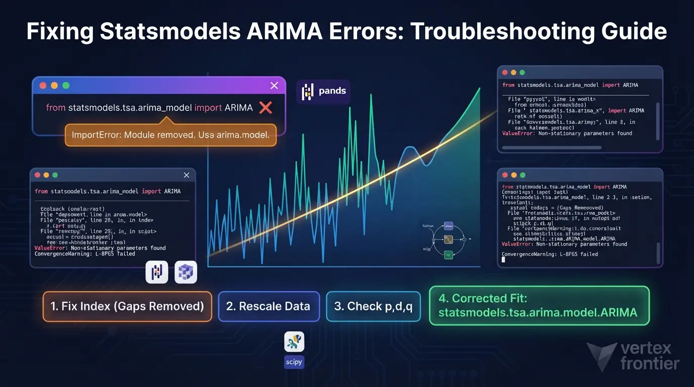

Your ARIMA fit crashed. Or it ran, printed an orange warning, and handed you a forecast that looks wrong.
Search for the error and the first answer is usually the same: set enforce_stationarity=False. That silences the message. It also removes the check that stops the optimizer from returning an explosive model. In a simulation built for this guide (an AR(1) fitted to 300 random walks of 100 observations), switching that check off produced an AR coefficient above 1 in 32% of the series.
That is the pattern behind most statsmodels ARIMA errors. The message blames the model. The cause sits upstream: the index, the scale, the data, or an import copied from an old tutorial.
This is a field manual, not a tutorial. For the modeling workflow itself, start with our Mastering ARIMA guide. Here you get what each failure means, what to try first, and what to avoid. statsmodels sits next to NumPy, SciPy and pandas in the Python data stack, and our guide to choosing a Python data library covers where it fits.
Every runnable code block below was executed on statsmodels 0.15.0, pandas 3.0.2, NumPy 2.4.4, SciPy 1.17.1 and Python 3.12. The catalog marks each error as reproduced or documented only, and a short evidence section near the end lists what each experiment does and does not prove.
Key takeaways
Click any topic to expand or collapseTo reproduce the results, pin the same versions:
Bash:
pip install "statsmodels==0.15.0" "pandas==3.0.2" "numpy==2.4.4" "scipy==1.17.1" python -c "import statsmodels, pandas; print(statsmodels.__version__, pandas.__version__)" The Import That No Longer Exists
A broken ARIMA script can fail on the very first model line.
For years, tutorials used from statsmodels.tsa.arima_model import ARIMA. That class is gone. The module still imports, so nothing looks wrong until you build a model.
What is the difference between statsmodels.tsa.arima_model.ARIMA and statsmodels.tsa.arima.model.ARIMA?
The first is a removed class: importing it works, but creating a model raises NotImplementedError. The second, with a dot between arima and model, is the current class. It runs on the state-space framework with a Kalman filter and subclasses SARIMAX.
Python Code:
 import statsmodels, pandas, numpy, scipy print("statsmodels", statsmodels.__version__) print("pandas", pandas.__version__, "| numpy", numpy.__version__, "| scipy", scipy.__version__)
from statsmodels.tsa.arima_model import ARIMA as OldARIMA # the import still succeeds... try: OldARIMA([1.0, 2.0, 3.0], order=(1, 1, 1)) # ...the constructor does not except NotImplementedError as exc: print("NotImplementedError:", " ".join(str(exc).split())[:140], "...")
Output:
statsmodels 0.15.0 pandas 3.0.2 | numpy 2.4.4 | scipy 1.17.1 NotImplementedError: statsmodels.tsa.arima_model.ARMA and statsmodels.tsa.arima_model.ARIMA have been removed in favor of statsmodels.tsa.arima.model.ARIMA (note ... The removal stub in the v0.13.5 source shows the old classes already raising by then, and the stub points to the new class. Older tutorials describe the class as “deprecated”. On a current install, that wording is out of date: the class is removed.
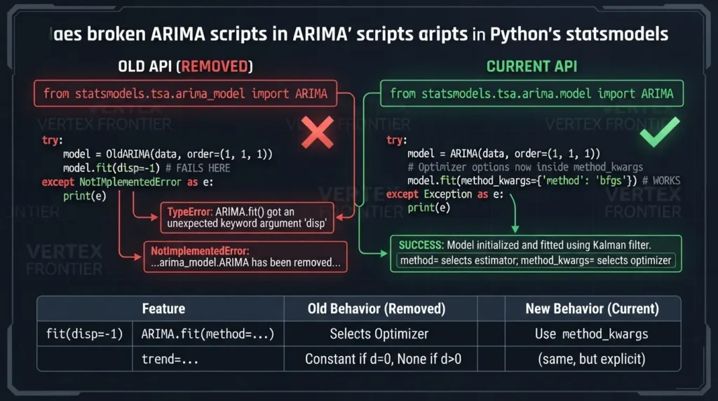
Switching the import is not enough. Four things change with it:
fit()takes different arguments.fit(disp=-1)from old tutorials raisesTypeError: ARIMA.fit() got an unexpected keyword argument 'disp'. Optimizer options now go insidemethod_kwargs.- In
ARIMA.fit, method=picks an estimator, not an optimizer. The valid values arestatespace(the default),innovations_mle, hannan_rissanen,burg,innovationsandyule_walker. InSARIMAX.fit, by contrast,method=is the optimizer (the statsmodels FAQ notebook callsSARIMAX(...).fit(method="bfgs")). Code that works on one class fails on the other. - The default trend depends on
d. It is a constant whend=0and none whend>0. trendis a regression term. That changes whatconstmeans. A later section covers it.
The statsmodels ARIMA documentation lists the full constructor.
| Behavior | On the tested stack | Note |
|---|---|---|
from statsmodels.tsa.arima_model import ARIMA | Import succeeds. Constructor raises NotImplementedError. | Removal stub present in v0.13.5 source. |
ARIMA.fit(method=...) | Selects an estimator: statespace (default), innovations_mle, hannan_rissanen, burg, innovations, yule_walker. | Not an optimizer name. |
method_kwargs={'method': 'bfgs'} | Selects the optimizer for the statespace fit. | Also accepts maxiter, disp. |
trend=None | Constant when d = 0, none when d > 0. | Checked from fitted parameter names. |
'M', 'Q', 'Y', 'A', 'BA', 'H', 'T', 'S' | Rejected by pandas 3.0.2. | Deprecated in pandas 2.2. |
SARIMAX.fit(method='bfgs') | Valid: in SARIMAX, method is the optimizer. | In ARIMA.fit the same call raises ValueError. |
Non-stationary / non-invertible ValueError | Raised after non-statespace estimators only. | Source, statsmodels tests, experiment. |
statsmodels.tsa.arima_model, switch to statsmodels.tsa.arima.model. The new class is a different model, not a renamed one.Fix the Data Before You Blame the Model
Here is the claim this guide keeps coming back to: when an ARIMA fit raises, check your data first and the model second.
Most articles start from the API. Start from the index instead. Four prerequisites prevent a large share of the errors people post about:
- A
DatetimeIndexthat is sorted and has no duplicate timestamps. - A regular frequency, so every period exists as a row.
- A deliberate policy for gaps: interpolate, forward-fill, or stop.
- A sane scale, which matters more than most guides admit (see the convergence section).

What statsmodels does with each kind of index
The surprise is that fit() accepts almost anything. The damage shows up later, when you forecast. Many readers see “the model fit fine” and assume the index is fine.
| Index you pass | fit() | forecast(steps=3) | forecast(‘date’) |
|---|---|---|---|
Regular dates, freq=None | Works. ValueWarning: inferred frequency used. | Works | Works |
| Gappy dates (missing periods) | Works. ValueWarning: index ignored. | ValueError: No supported index is available | KeyError: argument could not be matched |
| Integer RangeIndex | Works | Works (integer labels) | KeyError |
| NumPy array | Works | Works (returns an ndarray) | Not applicable |
| Duplicate timestamps | Works. ValueWarning: index ignored. | Not tested | asfreq() fails: duplicate labels |
These outcomes come from statsmodels 0.15.0 and pandas 3.0.2; other versions may word or handle them differently. Two rows deserve a closer look.
A regular index without a stored frequency is forgiven: statsmodels infers the frequency and warns. A gappy index is not forgiven. The fit succeeds with a ValueWarning, then both forecast(steps=3) and a date-string forecast fail. The statsmodels forecasting guide says date-based forecasting needs an index with a defined frequency.
Python Code:
 import warnings import numpy as np, pandas as pd from statsmodels.tsa.arima.model import ARIMA warnings.simplefilter("ignore")
full = pd.Series(np.cumsum(np.random.default_rng(1).standard_normal(120)) + 50, index=pd.date_range("2018-01-01", periods=120, freq="MS")) gappy = full.drop(full.index[[5, 6, 20]]) # three missing months -> irregular index print("freq:", gappy.index.freq, "| inferred:", gappy.index.inferred_freq)
res = ARIMA(gappy, order=(1, 1, 1), trend="t").fit() # the fit "works"... for label, call in [("forecast(steps=3)", lambda: res.forecast(steps=3)), ("forecast('2028-12-01')", lambda: res.forecast("2028-12-01"))]: try: call() except (ValueError, KeyError) as exc: # ...the forecast does not print(f"{label:24s} -> {type(exc).name}: {str(exc)[:70]}")
fixed = gappy.asfreq("MS").interpolate(limit=3) # regular index, short gaps interpolated res = ARIMA(fixed, order=(1, 1, 1), trend="t").fit() print(res.forecast("2028-03-01")) # date strings now resolve
Output:
freq: None | inferred: None forecast(steps=3) -> ValueError: No supported index is available. forecast('2028-12-01') -> KeyError: 'The `end` argument could not be matched to a location related to the 2028-01-01 43.419905 2028-02-01 43.110413 2028-03-01 42.854122 Freq: MS, Name: predicted_mean, dtype: float64 steps to dodge the KeyError”. On this stack that only helps if the index is regular or a plain integer index. With a gappy DatetimeIndex, forecast(steps=3) raises ValueError: No supported index is available. Repair the index instead.How to set up a DatetimeIndex for statsmodels ARIMA
- Parse, sort and de-duplicate. Convert strings with
pd.to_datetime, sort by date, and drop repeated timestamps.asfreq()refuses an index with duplicates. - Impose the frequency. Call
series.asfreq("MS")(or"D","B", and so on). Missing periods appear asNaN. - Decide what a gap means. Interpolate short gaps, forward-fill if the last value truly persists, or stop and investigate long ones.
The helper below does all three, and refuses to continue with an empty series. The demo input is deliberately messy: a duplicate row and two missing months.
Python Code:
 import pandas as pd
def prepare_series(df, date_col, value_col, freq, fill="interpolate", max_gap=3): """Turn a messy table into a regular, gap-aware series that statsmodels accepts.""" s = (df[[date_col, value_col]] .assign(**{date_col: lambda d: pd.to_datetime(d[date_col])}) .dropna(subset=[date_col]) .sort_values(date_col) .drop_duplicates(subset=date_col, keep="last") # asfreq() fails on duplicates .set_index(date_col)[value_col] .astype(float))
regular = s.asfreq(freq)                                 # inserts NaN rows for missing periods
n_gaps = int(regular.isna().sum())
print(f"{len(s)} observations -> {len(regular)} periods, {n_gaps} gap(s) filled with NaN")

if fill == "interpolate":
    regular = regular.interpolate(limit=max_gap, limit_area="inside")
elif fill == "ffill":
    regular = regular.ffill(limit=max_gap)
regular = regular.dropna()                               # leading/trailing leftovers
if regular.empty:
    raise ValueError("Series is empty after cleaning - check the date and value columns.")
return regular.asfreq(freq)                              # keep freq if gaps remain at the edges

--- demo on deliberately messy data ---------------------------------------
raw = pd.DataFrame({ "date": ["2024-01-01", "2024-02-01", "2024-02-01", "2024-04-01", "2024-05-01", "2024-07-01"], "sales": [100, 104, 105, 112, 115, 121], }) y = prepare_series(raw, "date", "sales", freq="MS") print(y.index.freq, "| NaNs left:", y.isna().sum())
Output:
5 observations -> 7 periods, 2 gap(s) filled with NaN <MonthBegin> | NaNs left: 0 For stock-style data, use "B" (business days). Holidays become NaN rows, so you still need a gap policy. If calendar gaps carry no meaning, a plain integer index is a legitimate choice. You give up date labels and date-string forecasts, and nothing else breaks.
If your raw table has millions of rows before resampling, do the resampling before the fit. When that step crawls, see why pandas is slow and how to fix it.
The pandas frequency alias trap
Frequency strings changed under people’s feet. The pandas change that renamed M to ME arrived as a deprecation in pandas 2.2. A later pandas pull request enforced that deprecation for M, Q, Y and related aliases, so on pandas 3.0.2 the old strings are rejected outright. The pandas time series documentation lists the current offsets.
Frequency alias cheat sheet (pandas 3.0.2)
| Old alias | Use now | Old alias on 3.0.2 |
|---|---|---|
| M (month end) | ME | Error |
| Q (quarter end) | QE | Error |
| Y or A (year end) | YE | Error |
| BA (business year end) | BYE | Error |
| H (hour) | h | Error |
| T (minute) | min | Error |
| S (second) | s | Error |
| MS, QS, YS, B, D | Unchanged | Works |
Results come from calling pd.date_range with each string on pandas 3.0.2. The pandas pull requests cited above cover M, Q, Y, H, T and S; BA and BYE were tested locally only.
The Error Catalog: Find Yours in 30 Seconds
What are the most common statsmodels ARIMA errors and their root causes?
- NotImplementedError: you imported the removed
arima_modelclass. - ValueError, non-stationary or non-invertible: a non-statespace estimator returned parameters the guards reject.
- ConvergenceWarning: the optimizer stopped before finding a solution, often because of scale or an over-sized model.
- ValueError, trend: a constant or “
ct” trend combined withd > 0. - KeyError or ValueError on forecast: a missing or irregular date frequency.
- ValueError on exog: missing or wrongly shaped future regressors.
- LinAlgError: a numerical failure in large or badly conditioned specifications.

Use the decoder to match a message. The table beneath it holds the same entries for scanning.
| Message | Root cause | First fix | Evidence |
|---|---|---|---|
| NotImplementedError: arima_model … have been removed | You built a model from the removed arima_model module. | from statsmodels.tsa.arima.model import ARIMA. Then re-check trend and fit() arguments. | Reproduced |
| TypeError: fit() got an unexpected keyword argument ‘disp’ | Old fit() arguments do not exist in the new class. | Move optimizer options into method_kwargs, e.g. method_kwargs={‘disp’: False, ‘maxiter’: 200}. | Reproduced |
| ValueError: Non-stationary autoregressive parameters found | A non-statespace estimator (e.g. hannan_rissanen) returned AR roots inside the unit circle. | Use the default method=’statespace’. If the data is non-stationary, raise d. Relax the guard last. | Reproduced |
| ValueError: Non-invertible moving average parameters found | A non-statespace estimator returned MA roots on or inside the unit circle, often from over-differencing. | Use method=’statespace’, lower q, and check that you did not difference twice. | Reproduced |
| ConvergenceWarning: Maximum Likelihood optimization failed to converge | The optimizer stopped before converging. With the default L-BFGS, warnflag 1 is an iteration or call limit and 2 is another stop reason such as a line-search failure. Tiny-variance data and over-sized models are common triggers. | Print res.mle_retvals and read warnflag for that optimizer. Limit flag: raise maxiter. Other flag: rescale (e.g. returns x 100), rotate optimizer, shrink order. | Reproduced |
| ValueError: In models with integration (d > 0) … trend terms | Differencing removes a constant, so a constant or ‘ct’ trend is rejected when d + D > 0. | Use trend=’t’ or ‘n’ when d = 1. For d = 2 use a quadratic polynomial such as [0, 0, 1]. | Reproduced |
| ValueError: No supported index is available | Gappy (irregular) DatetimeIndex: the fit worked, but forecasting cannot label the future. | series.asfreq(freq), then interpolate or fill short gaps. | Reproduced |
| KeyError: The `end` argument could not be matched to a location | A date-string forecast or predict on an index without a usable frequency (irregular dates or a RangeIndex). | Repair the index and set a frequency, or use an integer horizon on a regular or integer index. | Reproduced |
| ValueWarning: A date index has been provided, but it has no associated frequency | The DatetimeIndex has no stored frequency and could not be inferred. | asfreq() with the correct alias, then confirm series.index.freq is not None. | Reproduced |
| ValueError: Out-of-sample operations … require additional exogenous values | The model was fit with exog, but you forecast without future regressors. | Pass exog with one row per forecast step. | Reproduced |
| ValueError: Provided exogenous values are not of the appropriate shape | The future exog has the wrong number of rows or columns. | Match rows to steps and columns to the fit-time exog. | Reproduced |
| ValueError: Invalid frequency: M (pandas 3) | Pandas renamed aliases. Old ones were deprecated in 2.2 and are rejected on pandas 3.0.2. | Use ME, QE, YE, BYE, h, min, s. MS and QS are unchanged. | Reproduced |
| TypeError: object of type ‘numpy.float64’ has no len() | endog was a scalar instead of a 1-D series. | Pass a pd.Series or 1-D array. Check np.ndim(y) == 1. | Reproduced |
| LinAlgError: LU decomposition error | Numerical failure in large or badly conditioned specifications. Root cause not confirmed on this stack. | Shrink seasonal terms, rescale, raise d. AutoGluon documents raising d or enforce_stationarity=False. | Documented |
| LinAlgError: SVD did not converge | Too many parameters for the data, bad scaling, or near-duplicate exog columns. | Reduce order, rescale, inspect exog correlations. | Documented |
| EstimationWarning: Non-stationary starting autoregressive parameters | Not an error. statsmodels replaces bad starting values with zeros. | Ignore unless the fit then fails to converge. | Reproduced |
Three notes before the deep dives:
EstimationWarning: Non-stationary starting autoregressive parametersis not an error. statsmodels replaces bad starting values with zeros and carries on. It matters only if the fit then fails to converge.- Wrappers can bury the real message. If
pmdarima.auto_arimaor another wrapper fails, reproduce the failure with a plainARIMAcall first. That is a debugging habit, not a documented guarantee, but it usually shows the underlying exception. arma_order_select_icis not a safe order search. Its source (checked in 0.15.0) fits (p,0,q) only, supports only the"n"and"c"trends, and storesNaNfor any failed fit without telling you which one or why.
The “Non-stationary” and “Non-invertible” ValueErrors
This is the error with the worst folk remedy.
What is enforce_stationarity in statsmodels ARIMA?
It is a flag that restricts the AR parameters to values that describe a stationary process, meaning all AR roots lie outside the unit circle. enforce_invertibility does the same for the MA side. Both default to True, and they exist to keep forecasts from exploding.

Here is the part most guides miss. On the default estimator, you almost never see these ValueErrors. The default method="statespace” optimizes in a transformed space where every candidate is already stationary. The exceptions are raised in the ARIMA source after a non-statespace estimator returns its answer. The statsmodels own test suite asserts this behavior for Hannan-Rissanen. That is also the estimator the example below uses, so treat Hannan-Rissanen as the confirmed case.
Python Code:
 import warnings, numpy as np, pandas as pd from statsmodels.tsa.arima.model import ARIMA warnings.simplefilter("ignore")
rng = np.random.default_rng(5) walk = pd.Series(np.cumsum(rng.standard_normal(120)), index=pd.date_range("2020-01-01", periods=120, freq="D"))
try: # a non-MLE estimator does not constrain its answer ARIMA(walk, order=(1, 0, 1), trend="n").fit(method="hannan_rissanen") except ValueError as exc: print("ValueError:", exc)
res = ARIMA(walk, order=(1, 0, 1), trend="n").fit() # default: method="statespace" print("statespace fit works. converged =", res.mle_retvals["converged"])
Output:
ValueError: Non-stationary autoregressive parameters found with `enforce_stationarity=True`. Consider setting it to False or using a different estimation method, such as method="statespace". statespace fit works. converged = True Read the message again. It suggests method="statespace". That is the first fix, and it is not the one Stack Overflow leads with.
Why switching the guard off is the wrong first move
“Wrong” here is measurable. The experiment below fits an AR(1) with the guard on and off to 300 simulated random walks of 100 observations each, then forecasts 100 steps ahead. Random walks are the worst case, since their true root is exactly 1. Price-like series are a reasonable stress test, but this experiment does not measure any real dataset.
Python Code:
 # Experiment 1: how often does disabling enforce_stationarity give an explosive AR root? import warnings, numpy as np, pandas as pd from statsmodels.tsa.arima.model import ARIMA warnings.simplefilter("ignore")
N_SERIES, N_OBS, H = 300, 100, 100 explosive, big_gap, gaps = 0, 0, [] for seed in range(N_SERIES): rng = np.random.default_rng(seed) y = pd.Series(np.cumsum(rng.standard_normal(N_OBS)), index=pd.date_range("2020-01-01", periods=N_OBS, freq="D")) on = ARIMA(y, order=(1, 0, 0), trend="n").fit() off = ARIMA(y, order=(1, 0, 0), trend="n", enforce_stationarity=False).fit() if off.params["ar.L1"] > 1.0: explosive += 1 gap = abs(float(off.forecast(H).iloc[-1]) - float(on.forecast(H).iloc[-1])) gaps.append(gap) gaps = np.array(gaps) print(f"series: {N_SERIES}, obs each: {N_OBS}, horizon: {H}") print(f"guard OFF gave phi > 1 in {explosive} series ({explosive/N_SERIES:.0%})") print(f"median |forecast gap| at h={H}: {np.median(gaps):.2f}") print(f"95th pct gap: {np.percentile(gaps,95):.2f}, max gap: {gaps.max():.2f}")
Output:
series: 300, obs each: 100, horizon: 100 guard OFF gave phi > 1 in 96 series (32%) median |forecast gap| at h=100: 1.34 95th pct gap: 57.04, max gap: 180.22 The median difference is small. The tail is the problem. In one series in twenty, the guarded and unguarded forecasts differ by 57 units or more, where the random-walk step is 1. You will not see this on the series you tested. You will see it on the one that runs in production at 3 a.m.
The safer repair order:
- Verify stationarity. Run ADF and KPSS together; our KPSS test guide explains how to read disagreements between them.
- Raise
dby one if the tests say the level is not stationary. - Lower
porq. Redundant parameters push roots toward the boundary. - Use the default
statespaceestimator. - Only then relax the guard, with a comment explaining why, and compare the forecast against a hold-out period.
A quick boundary check
For the simplest models the rule is short. An AR(1) is stationary when the absolute value of phi is below 1. An MA(1) is invertible when the absolute value of theta is below 1. Higher orders need all roots checked; after a fit, res.arroots and res.maroots give them, and every modulus should exceed 1.
Result appears here.
The LU decomposition and SVD errors
numpy.linalg.LinAlgError: LU decomposition error is the guard family’s awkward cousin. The documentation for AutoGluon’s ARIMA wrapper says that if it crashes with this error, you can set enforce_stationarity to False or increase d. That is a documented workaround from a library that wraps statsmodels for automated forecasting.
This error did not trigger on synthetic data on the tested stack, so the table marks it documented. Treat the root cause as unconfirmed. In practice, try these in order:
- Shrink the specification, especially seasonal AR and MA terms.
- Rescale the series.
- Raise
d. - Relax the guard, and log that you did.
LinAlgError: SVD did not converge has the same shape: too many parameters for too little data, badly scaled values, or exogenous columns that are near-duplicates of each other. Check the exog correlation matrix before you touch the order.
ConvergenceWarning and the mle_retvals You Were Told to Check
The warning ends with “Check mle_retvals”. Few pages say how.
How to fix ConvergenceWarning: Maximum Likelihood optimization failed to converge in statsmodels ARIMA:
- Print
res.mle_retvalsand readconverged,warnflagand which optimizer ran. - Translate
warnflagfor that optimizer. With the default L-BFGS, 1 means an iteration or function-call limit, and 2 means it stopped for another reason, often a line-search failure. - Limit flag: raise
maxiterthroughmethod_kwargs. Other-reason flag: rescale the series, then try another optimizer. - If it still fails, reduce the model order or change the specification.
The state-space fit defaults to 50 iterations, which explains most limit flags. A flag that means “stopped for another reason” will not be cured by a bigger maxiter, so a loop that raises it to 10,000 is solving the wrong problem.

Flag numbers are not universal. The SciPy documentation for fmin_powell uses 1 for the function-call limit and 2 for the iteration limit, while BFGS uses 2 for a precision loss. Always read the flag against the optimizer that produced it.
What mle_retvals actually contains
The keys depend on the optimizer. There is no message key on the default one.
| Optimizer | Keys in mle_retvals (observed) | What warnflag means (SciPy docs) |
|---|---|---|
| lbfgs (default) | converged, warnflag, iterations, fcalls, fopt, gopt | 1: iteration or call limit. 2: stopped for another reason (often line search). |
| bfgs | converged, warnflag, fcalls, gcalls, fopt, gopt, Hinv | 1: iteration limit. 2: precision loss. 3: NaN. |
| powell | converged, warnflag, iterations, fcalls, fopt, direc | 1: function-call limit. 2: iteration limit. 3: NaN. 4: out of bounds. |
| nm (Nelder-Mead) | converged, warnflag, iterations, fcalls, fopt | 1: function-call limit. 2: iteration limit. |
Python Code:
 import warnings, numpy as np, pandas as pd from statsmodels.tsa.arima.model import ARIMA
warnflag means different things for different optimizers (see scipy.optimize docs)
FLAGS = { "lbfgs": {1: "iteration or function-call limit", 2: "stopped for another reason, often a line-search failure"}, "bfgs": {1: "iteration limit", 2: "gradient or function stopped changing (precision loss)", 3: "NaN encountered"}, "powell": {1: "function-call limit", 2: "iteration limit", 3: "NaN encountered", 4: "result out of bounds"}, "nm": {1: "function-call limit", 2: "iteration limit"}, }
def convergence_report(res): """Plain-English summary of res.mle_retvals for the optimizer that was actually used.""" r = res.mle_retvals if r is None: return "No mle_retvals: this estimator is not an iterative optimizer." opt = (res.mle_settings or {}).get("optimizer") or "lbfgs" # None means the default, lbfgs flag = r.get("warnflag") meaning = "converged" if flag == 0 else FLAGS.get(opt, {}).get(flag, "see scipy.optimize docs") return (f"optimizer={opt} | converged={r.get('converged')} | warnflag={flag} ({meaning}) | " f"iterations={r.get('iterations', 'n/a')} | function calls={r.get('fcalls')}")
Same data, two scales: raw log returns vs percent returns
rng = np.random.default_rng(3) returns = pd.Series(0.01 * rng.standard_normal(250), index=pd.bdate_range("2023-01-02", periods=250))
with warnings.catch_warnings(): warnings.simplefilter("ignore") raw = ARIMA(returns, order=(1, 0, 0)).fit() scaled = ARIMA(returns * 100, order=(1, 0, 0)).fit()
print("raw scale :", convergence_report(raw)) print("x100 scale:", convergence_report(scaled)) print("raw keys :", sorted(raw.mle_retvals))
Output:
raw scale : optimizer=lbfgs | converged=False | warnflag=2 (stopped for another reason, often a line-search failure) | iterations=1 | function calls=168 x100 scale: optimizer=lbfgs | converged=True | warnflag=0 (converged) | iterations=4 | function calls=24 raw keys : ['converged', 'fcalls', 'fopt', 'gopt', 'iterations', 'warnflag'] The same data, multiplied by 100, converged in 4 iterations. The raw series quit after one, with flag 2 on the default optimizer.
Scale is the hidden cause
Daily log returns have a standard deviation near 0.01, so the variance is near 0.0001. The likelihood surface is flat at that scale, and the optimizer’s line search gives up. To measure how often, the experiment below fits 200 simulated return series of 250 observations, raw and multiplied by 100 (percent returns).
Python Code:
import warnings, numpy as np, pandas as pd from statsmodels.tsa.arima.model import ARIMA from statsmodels.tools.sm_exceptions import ConvergenceWarning N_SERIES, N_OBS = 200, 250 def run(label, scale, order): cw = 0; ex = None for seed in range(N_SERIES): rng = np.random.default_rng(seed) idx = pd.bdate_range("2023-01-02", periods=N_OBS) r = pd.Series(0.01*rng.standard_normal(N_OBS), index=idx) * scale # log-returns, scaled with warnings.catch_warnings(record=True) as w: warnings.simplefilter("always") res = ARIMA(r, order=order, trend="c").fit() bad = any(issubclass(x.category, ConvergenceWarning) for x in w) or not res.mle_retvals["converged"] cw += bad if bad and ex is None: ex = (seed, res.mle_retvals["warnflag"], res.mle_retvals["iterations"]) print(f"{label:34s} failures={cw:3d}/{N_SERIES} ({cw/N_SERIES:.1%}) first_bad(seed,warnflag,iters)={ex}") run("returns x1 (sigma2~1e-4) AR(1)", 1, (1,0,0)) run("returns x100 (sigma2~1) AR(1)", 100, (1,0,0)) run("returns x1 ARMA(1,1)", 1, (1,0,1)) run("returns x100 ARMA(1,1)", 100, (1,0,1)) run("returns x1 (0,0,0)", 1, (0,0,0)) run("returns x100 (0,0,0)", 100, (0,0,0)) Output:
returns x1 (sigma2~1e-4) AR(1) failures= 21/200 (10.5%) first_bad(seed,warnflag,iters)=(3, 2, 1) returns x100 (sigma2~1) AR(1) failures= 0/200 (0.0%) first_bad(seed,warnflag,iters)=None returns x1 ARMA(1,1) failures= 16/200 (8.0%) first_bad(seed,warnflag,iters)=(28, 2, 1) returns x100 ARMA(1,1) failures= 1/200 (0.5%) first_bad(seed,warnflag,iters)=(73, 1, 50) returns x1 (0,0,0) failures= 6/200 (3.0%) first_bad(seed,warnflag,iters)=(4, 2, 5) returns x100 (0,0,0) failures= 0/200 (0.0%) first_bad(seed,warnflag,iters)=None An uncommon insight sits in these numbers. A tempting hypothesis says ARIMA on prices breaks convergence and returns fix it. The simulation did not support that. On simulated random-walk prices, ARIMA(1,1,1) produced a convergence failure in 0 of 200 fits with trend="n" and 4 of 200 with trend="t". Returns at their natural scale failed more often, not less. In this simulation the two clear culprits were scale and redundancy: in 193 of 200 price fits (96%), the fitted AR and MA coefficients nearly cancelled each other (|phi + theta| under 0.15). When the data is a random walk, ARIMA(1,1,1) has two parameters that explain nothing.
Model returns if returns are what you care about. Just don’t expect that choice alone to cure a ConvergenceWarning. These are simulated Gaussian series, so the numbers show a mechanism, not the failure rate of your data.
Which optimizer to try
| Optimizer | Function calls on one 120-point example | When to use |
|---|---|---|
| lbfgs | 100 | Default. Start here, with scaled data. |
| bfgs | 21 (+21 gradient) | First fallback. |
| powell | 146 | Try when gradients mislead. |
| nm | 291 | Last in the rotation. Slow but forgiving. |
Optimizer rotation helps when the surface is awkward rather than flat. A later section builds it into a safe fitting function.
fit(method="bfgs") does not select the BFGS optimizer. It raises ValueError: estimator must be one of: 'yule_walker', 'burg', 'innovations', 'hannan_rissanen', 'innovations_mle', 'statespace'. The optimizer goes in method_kwargs={"method": "bfgs"}.warnflag against the optimizer that produced it before changing anything. On the default L-BFGS, a limit flag asks for iterations and an "other reason" flag asks for rescaling or a smaller model.Trend and Differencing: Why trend=”c” Fails When d > 0
The message is long and the logic is short.
ValueError: In models with integration (d > 0) or seasonal integration (D > 0), trend terms of lower order than d + D cannot be included...
Differencing a series once removes a constant. If you add a constant back, it has nothing to estimate. A linear trend in the levels, on the other hand, becomes a constant in the differences. That is why trend="t" is the legal substitute: it plays the role of the constant of the differenced data.

The test below fits every combination of d and trend. Nothing here is theory; the code printed it.
Python Code:
 import numpy as np, pandas as pd from statsmodels.tsa.arima.model import ARIMA
rng = np.random.default_rng(0) y = pd.Series(np.cumsum(rng.standard_normal(120)) + 50, index=pd.date_range("2018-01-01", periods=120, freq="MS"))
for d in (0, 1): for trend in ("n", "c", "t", "ct"): try: ARIMA(y, order=(1, d, 1), trend=trend).fit() status = "ok" except ValueError: status = "ValueError" print(f"d={d} trend={trend!r:5} {status}")
d=2 needs a trend polynomial of order >= 2, i.e. a quadratic term:
ARIMA(y, order=(1, 2, 1), trend=[0, 0, 1]).fit() print("d=2 trend=[0, 0, 1] ok")
Output:
d=0 trend='n' ok d=0 trend='c' ok d=0 trend='t' ok d=0 trend='ct' ok d=1 trend='n' ok d=1 trend='c' ValueError d=1 trend='t' ok d=1 trend='ct' ValueError d=2 trend=[0, 0, 1] ok | Differencing | trend=’n’ | trend=’c’ | trend=’t’ | trend=’ct’ |
|---|---|---|---|---|
| d = 0 | ok | ok | ok | ok |
| d = 1 | ok | ValueError | ok | ValueError |
| d = 2 | ok | ValueError | ValueError (use [0, 0, 1]) | ValueError |
d=2, the trend polynomial must reach order 2 or higher, so trend="t" will fail too. The example above passes [0, 0, 1], a pure quadratic term. If you reach for a quadratic trend, ask whether twice-differenced data is really what you want.Seasonal differencing counts as well. The rule uses d + D, so order=(1, 0, 1) with seasonal_order=(0, 1, 1, 12)also rejects trend="c". Our SARIMA guide covers choosing D.
d > 0, use "n" or "t". Constants and "ct" are rejected.ARIMA vs SARIMAX: The Same Model With a Different const
Migrating code without reading the docs gets you here. The two classes agree on the AR coefficient and disagree on the number labeled as the constant.

The statsmodels SARIMAX and ARIMA FAQ explains why. In ARIMA, a trend or intercept behaves like a regression term with ARMA errors, so const is the long-run mean. In SARIMAX, the intercept sits inside the ARMA recursion, so it is the conditional intercept. The SARIMAX class documentation defines that model.
For a stationary AR(1), the FAQ shows the two estimates agree in large samples. Here is the relationship on simulated data with a long-run mean of 10:
Python Code:
 import numpy as np, pandas as pd from statsmodels.tsa.arima.model import ARIMA from statsmodels.tsa.statespace.sarimax import SARIMAX
rng = np.random.default_rng(1) e = rng.standard_normal(400) y = np.zeros(400) for t in range(1, 400): # AR(1) with long-run mean 10, phi = 0.7 y[t] = 3.0 + 0.7 * y[t - 1] + e[t] y = pd.Series(y, index=pd.date_range("2015-01-01", periods=400, freq="D"))
a = ARIMA(y, order=(1, 0, 0), trend="c").fit() s = SARIMAX(y, order=(1, 0, 0), trend="c").fit(disp=False)
phi = s.params["ar.L1"] print(f"ARIMA const = {a.params['const']:.3f} (the long-run mean)") print(f"SARIMAX intercept = {s.params['intercept']:.3f} (the conditional intercept)") print(f"intercept / (1 - phi) = {s.params['intercept'] / (1 - phi):.3f} <- matches ARIMA const")
Output:
ARIMA const = 9.596 (the long-run mean) SARIMAX intercept = 3.280 (the conditional intercept) intercept / (1 - phi) = 9.596 <- matches ARIMA const Result appears here.
The FAQ shows the same split on its own example: a constant near 9.77 in ARIMA, an intercept near 1.99 in SARIMAX, and a long-run mean near 9.77 in both. When someone says "my const changed after I switched models", check the class before you debug the code.
For models with exogenous regressors, the FAQ notes that the exog coefficients agree between the two classes while the intercept still differs.
Forecasting and exog Errors
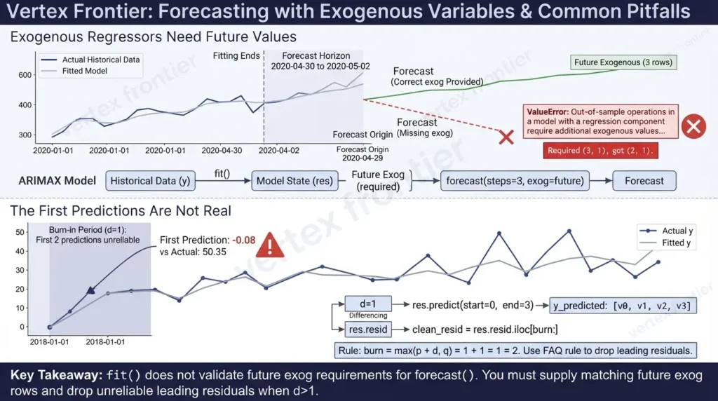
Fitting passes. Forecasting fails. The mental model most people hold is that fit() validates everything. It does not.
Exogenous regressors need future values
If you fit with exog, you must supply future exog rows for every forecast step. The error messages are clear once you know where to look.
Python Code:
 import numpy as np, pandas as pd from statsmodels.tsa.arima.model import ARIMA
rng = np.random.default_rng(1) idx = pd.date_range("2020-01-01", periods=120, freq="D") promo = pd.DataFrame({"promo": rng.integers(0, 2, 120)}, index=idx) # 2-D by construction y = pd.Series(50 + 3 * promo["promo"] + rng.standard_normal(120).cumsum() * 0.1, index=idx)
res = ARIMA(y, exog=promo, order=(1, 0, 0), trend="c").fit()
future = pd.DataFrame({"promo": [0, 1, 0]}, # must match the horizon index=pd.date_range(idx[-1] + pd.Timedelta(days=1), periods=3, freq="D")) for label, call in [("no exog", lambda: res.forecast(steps=3)), ("2 rows for 3 steps", lambda: res.forecast(steps=3, exog=future.iloc[:2]))]: try: call() except ValueError as exc: print(f"{label:20s} -> {str(exc)[:95]}")
print(res.forecast(steps=3, exog=future).round(2).to_string())
Output:
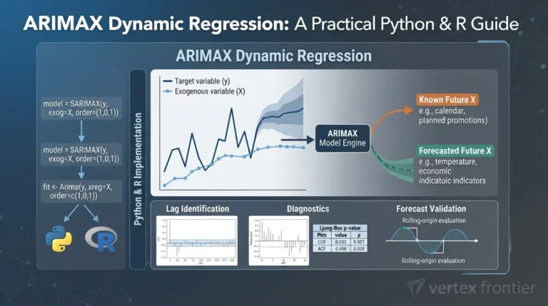
no exog -> Out-of-sample operations in a model with a regression component require additional exogenous va 2 rows for 3 steps -> Provided exogenous values are not of the appropriate shape. Required (3, 1), got (2, 1). 2020-04-30 48.82 2020-05-01 51.83 2020-05-02 48.85 Freq: D Build exog as a DataFrame so it is two-dimensional by construction. On this stack, a 1-D array was also accepted at fit time, but a DataFrame removes any shape guesswork. For lag selection and forecast leakage with exogenous variables, our ARIMAX dynamic regression guide goes deeper.
The first predictions are not real
With d=1, the first in-sample prediction is meaningless, and nothing warns you. The new API raises no error here. It just hands you a number:
Python Code:
 import warnings, numpy as np, pandas as pd from statsmodels.tsa.arima.model import ARIMA warnings.simplefilter("ignore")
y = pd.Series(np.cumsum(np.random.default_rng(1).standard_normal(120)) + 50, index=pd.date_range("2018-01-01", periods=120, freq="MS")) p, d, q = 1, 1, 1 res = ARIMA(y, order=(p, d, q), trend="t").fit()
fitted = res.predict(start=0, end=3) # in-sample one-step-ahead predictions print(pd.DataFrame({"actual": y.iloc[:4], "predicted": fitted}).round(2).to_string())
The statsmodels FAQ: residuals before max((P+D)s + p + d, Qs + q) are unreliable
burn = max(p + d, q) # no seasonal part here print("unreliable leading residuals:", burn, "| res.loglikelihood_burn:", res.loglikelihood_burn) clean_resid = res.resid.iloc[burn:] # use this for any error metric
Output:
actual predicted 2018-01-01 50.35 -0.08 2018-02-01 51.17 50.27 2018-03-01 51.50 50.99 2018-04-01 50.19 51.27 unreliable leading residuals: 2 | res.loglikelihood_burn: 1 The first prediction is about -0.08 against an actual 50.35. The statsmodels FAQ explains the cause: with no history, the best prediction of the first differenced value is the mean of the differences. It also gives a rule for how many leading residuals to distrust: max((P+D)*s + p + d, Q*s + q). For ARIMA(1,1,1) that is 2.
Use that rule for error metrics. statsmodels also exposes loglikelihood_burn and nobs_diffuse, but here loglikelihood_burn is 1, which is less conservative than the FAQ rule of 2.
Three Documented Cases
Real examples beat invented ones. The three below are documented in public sources. Where a source gives no measured outcome, the card says so.
Challenge: A brute-force search over regular and seasonal ARIMA orders for a 396-observation retail sales series hit failures.
Action: The Spring 2025 lecture notebook wrapped each fit in try/except and kept the rest of the results.
Outcome: One specification failed with LU decomposition error, several others warned about convergence, and the search still produced AIC and BIC winners.
Lesson: Failures are normal in order searches. Catch them and log them.
Challenge: An automated forecasting library built on statsmodels needed guidance for ARIMA crashes with LU decomposition errors.
Action: Its ARIMA documentation tells users to set enforce_stationarity to False or raise d.
Outcome: No measured result is published. Evidence here is limited to the documented guidance, and AutoGluon's model is built on SARIMAX, so treat it as guidance by analogy for ARIMA.
Lesson: Even library authors treat this as a specification problem, and list a higher d as one of two options.
Challenge: The same AR(1) with a constant gives very different numbers in ARIMA and SARIMAX.
Action: The official FAQ notebook fits both and compares them.
Outcome: A constant near 9.77 in ARIMA, an intercept near 1.99 in SARIMAX, and a long-run mean near 9.77 in both.
Lesson: Compare long-run means across classes, not raw intercepts.
The Berkeley lecture deserves a longer look. It runs a brute-force search over p, d, q and the seasonal orders for a 396-observation retail sales series, wrapping each fit in try/except. One specification failed with LU decomposition error, and several others emitted convergence warnings. The authors' own conclusion is that fitting these models is hard because it involves nonlinear optimization. The lesson is the try/except itself: the search still finished, and the failures were visible.
A Production Pattern: Fit Defensively, Log Everything
A crash is better than a silent bad forecast. The trouble with most "safe fit" snippets is that they swallow every failure and relax guards without telling anyone.
The version below rotates optimizers first, keeps guards on, records every attempt, and relaxes them only if you ask. It also fixes a bug worth knowing about: many templates pass the optimizer as fit(method="bfgs"), which raises ValueError and is then swallowed by an except ValueError, so only the default optimizer is ever tried.
Python Code:
 import warnings import numpy as np import pandas as pd from statsmodels.tsa.arima.model import ARIMA
SOLVERS = [None, "bfgs", "powell", "nm"] # None = statsmodels default (lbfgs)
def safe_arima_fit(y, order, trend=None, maxiter=500, allow_relaxed=False): """Fit ARIMA, rotate optimizers, and keep an audit trail.
Returns (results_or_None, log). Guards stay ON unless allow_relaxed=True,
and a relaxed fit is flagged in the log so it can never pass silently.
"""
log = []
attempts = [(s, True) for s in SOLVERS]
if allow_relaxed:
    attempts += [(s, False) for s in SOLVERS[:2]]  # last resort, guards off

for solver, guards in attempts:
    kwargs = {"maxiter": maxiter}
    if solver:
        kwargs["method"] = solver                  # optimizer goes INSIDE method_kwargs
    try:
        with warnings.catch_warnings():
            warnings.simplefilter("ignore")
            res = ARIMA(y, order=order, trend=trend,
                        enforce_stationarity=guards,
                        enforce_invertibility=guards).fit(method_kwargs=kwargs)
        ok = bool(res.mle_retvals.get("converged", False))
        log.append(dict(solver=solver or "lbfgs", guards=guards, converged=ok))
        if ok:
            res.guards_relaxed = not guards
            return res, log
    except (ValueError, np.linalg.LinAlgError) as exc:
        log.append(dict(solver=solver or "lbfgs", guards=guards,
                        error=f"{type(exc).__name__}: {str(exc)[:60]}"))
return None, log

--- usage: a series where the default optimizer (lbfgs) gives up ---
returns = pd.Series(0.01 * np.random.default_rng(3).standard_normal(250), index=pd.bdate_range("2023-01-02", periods=250))
res, log = safe_arima_fit(returns, order=(1, 0, 0), trend="c") for row in log: print(row) print("guards relaxed:", res.guards_relaxed)
Output:
{'solver': 'lbfgs', 'guards': True, 'converged': False} {'solver': 'bfgs', 'guards': True, 'converged': True} guards relaxed: False The default optimizer failed on the raw-scale returns. BFGS succeeded. The log shows both, so you can see why the fit worked. Rescaling would have fixed it with the default optimizer, which is the cleaner remedy.
asfreq(), choose a gap policy.mle_retvals and the optimizer. A limit flag: raise maxiter. Any other flag: go to step 5.Replace arma_order_select_ic with a search that tells you what failed
The same try/except idea gives you an order search that returns a failure log. Note the trend switch: "c" for d=0, "t" once d>0.
Python Code:
 import itertools, warnings import numpy as np, pandas as pd from statsmodels.tsa.arima.model import ARIMA
def order_search(y, max_p=2, max_d=1, max_q=2, trend_for_d0="c"): """Manual AIC search that records failures instead of crashing.""" rows, failures = [], [] for p, d, q in itertools.product(range(max_p + 1), range(max_d + 1), range(max_q + 1)): trend = trend_for_d0 if d == 0 else "t" # 'c' is illegal once d > 0 try: with warnings.catch_warnings(): warnings.simplefilter("ignore") res = ARIMA(y, order=(p, d, q), trend=trend).fit() if res.mle_retvals.get("converged", False): rows.append(dict(p=p, d=d, q=q, aic=res.aic, bic=res.bic)) else: failures.append(((p, d, q), "did not converge")) except (ValueError, np.linalg.LinAlgError) as exc: failures.append(((p, d, q), f"{type(exc).name}: {str(exc)[:40]}")) table = pd.DataFrame(rows).sort_values("aic").reset_index(drop=True) return table, failures
y = pd.Series(np.cumsum(np.random.default_rng(4).standard_normal(150)) + 20, index=pd.date_range("2016-01-01", periods=150, freq="MS")) table, failures = order_search(y) print(table.head(3).round(2).to_string(index=False)) print(f"{len(table)} candidates kept, {len(failures)} rejected")
Output:
p d q aic bic 0 1 2 425.66 437.67 2 1 2 426.35 444.37 2 1 0 427.11 439.12 18 candidates kept, 0 rejected Two more production habits:
- Pin your versions. Behavior in this guide is version-specific. Record
statsmodels,pandasandNumPyin your lockfile, and re-run your fits when you upgrade. - Guard short groups in distributed jobs. A group with only a handful of rows cannot support the order you chose. Skip it or fall back to a simpler model instead of crashing the whole job. If you are structuring this code for a team, our scalable Python project structure guide helps.
Verify before you ship
A fit that converges is not a fit you can trust. Two small functions turn "it ran" into evidence: a post-fit checklist, and a hold-out comparison that justifies (or kills) any relaxed guard.
Python Code:
 import warnings, numpy as np, pandas as pd from statsmodels.tsa.arima.model import ARIMA from statsmodels.stats.diagnostic import acorr_ljungbox
def verify_fit(res, y, order, seasonal=(0, 0, 0, 0)): """Post-fit checklist. Returns {check: True/False}. Any False means: do not ship.""" (p, d, q), (P, D, Q, s) = order, seasonal burn = max((P + D) * s + p + d, Q * s + q) # unreliable leading residuals (statsmodels FAQ) resid = res.resid.iloc[burn:] if hasattr(res.resid, "iloc") else res.resid[burn:] lb_p = float(acorr_ljungbox(resid, lags=[10])["lb_pvalue"].iloc[0]) retvals = res.mle_retvals or {} return { "index has a frequency (or is a RangeIndex)": y.index.freq is not None or isinstance(y.index, pd.RangeIndex), "optimizer converged": bool(retvals.get("converged", True)), "guards were not relaxed": not getattr(res, "guards_relaxed", False), "AR roots outside the unit circle": bool(np.all(np.abs(res.arroots) > 1)), "MA roots outside the unit circle": bool(np.all(np.abs(res.maroots) > 1)), f"Ljung-Box p > 0.05 after dropping {burn} residuals": lb_p > 0.05, }
def holdout_check(y, order, trend, h=12): """RMSE on the last h points: guards on vs guards off vs a naive last-value forecast.""" train, test = y.iloc[:-h], y.iloc[-h:] rmse = lambda f: float(np.sqrt(np.mean((test.values - np.asarray(f)) ** 2))) out = {} with warnings.catch_warnings(): warnings.simplefilter("ignore") for label, guards in (("guards on", True), ("guards off", False)): res = ARIMA(train, order=order, trend=trend, enforce_stationarity=guards, enforce_invertibility=guards).fit() out[label] = rmse(res.forecast(h)) out["naive last value"] = rmse(np.repeat(train.iloc[-1], h)) return out
y = pd.Series(np.cumsum(np.random.default_rng(1).standard_normal(120)) + 50, index=pd.date_range("2018-01-01", periods=120, freq="MS")) with warnings.catch_warnings(): warnings.simplefilter("ignore") res = ARIMA(y, order=(1, 1, 1), trend="t").fit()
for check, ok in verify_fit(res, y, (1, 1, 1)).items(): print("PASS" if ok else "FAIL", "-", check) print({k: round(v, 2) for k, v in holdout_check(y, (1, 1, 1), "t").items()})
Output:
PASS - index has a frequency (or is a RangeIndex) PASS - optimizer converged PASS - guards were not relaxed PASS - AR roots outside the unit circle PASS - MA roots outside the unit circle PASS - Ljung-Box p > 0.05 after dropping 2 residuals {'guards on': 1.87, 'guards off': 2.07, 'naive last value': 1.4} Look at the last line. On this simulated random walk, the naive last-value forecast (RMSE 1.40) beat both ARIMA fits (1.87 with guards on, 2.07 with guards off). That is the point of a hold-out: a model that fits without errors can still lose to a forecast that needs no model. This is one simulated series, so read it as a demonstration of the method, not a verdict on ARIMA.
| Check | Why it matters | If it fails |
|---|---|---|
| Index has a frequency | Forecast labels and date strings need it. | Run asfreq() and choose a gap policy. |
| Optimizer converged | An unconverged fit has no trustworthy parameters. | Rescale, rotate optimizer, shrink order. |
| Guards were not relaxed | A relaxed fit needs a written reason. | Compare against the guarded model on a hold-out. |
| AR and MA roots outside the unit circle | Roots near 1 mean unstable or redundant terms. | Lower p or q, or raise d. |
| Ljung-Box after dropping leading residuals | Autocorrelated residuals mean missing structure. | Revisit the order, seasonality or exog. |
| Hold-out beats a naive forecast | A model that loses to last-value adds no signal. | Simplify, or do not deploy. |
What the Evidence Does and Does Not Show
Not every statement in this guide has the same strength. Each one falls in one of three classes:
- Documented: stated in official documentation or source code, such as the statsmodels FAQ, the ARIMA source, or the SciPy optimizer docs.
- Hands-on observation: observed on the tested stack under the conditions listed. It says nothing about other versions or your data.
- Editorial inference: a recommendation or interpretation. It is a judgment, not a vendor guarantee.
| Claim | Evidence class | Scope and limits |
|---|---|---|
Old arima_model constructor raises NotImplementedError | Documented + hands-on | v0.13.5 source stub; tested on 0.15.0. |
| Guard ValueErrors need a non-statespace estimator | Documented + hands-on | Source and statsmodels tests; reproduced with Hannan-Rissanen only. |
| 32% of random walks gave phi above 1 with the guard off | Hands-on observation | Simulation 1 only. Nothing about real data. |
| Rescaling returns by 100 cut convergence failures | Hands-on observation | Simulation 2 only. Gaussian returns, three small models. |
| Prices-versus-returns did not explain convergence failures | Hands-on observation | Simulation 3 only. Synthetic random-walk prices. |
| const versus intercept relation | Documented | statsmodels FAQ; holds in large samples. |
| Leading residuals to distrust | Documented | statsmodels FAQ formula. |
| warnflag meanings | Documented | SciPy docs, per optimizer. |
| LU and SVD LinAlgError causes | Documented, unconfirmed | Not triggered on the tested stack. |
| Gappy-index forecast failures | Hands-on observation | statsmodels 0.15.0, pandas 3.0.2. |
| Relax guards last; wrappers can bury errors | Editorial inference | Recommendation, not a vendor guarantee. |
The three simulations used these exact conditions:
| Run | Data-generating process | Size | Seeds | Models fitted | Metric |
|---|---|---|---|---|---|
| 1. Guard off | Gaussian random walk, step sd 1 | 300 series x 100 obs, horizon 100 | Seeds 0-299 | AR(1), trend n, guards on vs off | Share with phi above 1; forecast gap |
| 2. Scale | i.i.d. Gaussian returns, sd 0.01 | 200 series x 250 obs | Seeds 0-199 | AR(1), ARMA(1,1), constant only; raw vs x100 | Share with ConvergenceWarning or converged=False |
| 3. Prices | Random-walk prices 100*exp(cumsum(0.01 z)) | 200 series x 250 obs | Seeds 0-199 | ARIMA(1,1,1), trend n and t | Convergence failures; |phi+theta| under 0.15 |
None of these simulations measures a real dataset. They show mechanisms you can check on your own data with the code above.
Common Mistakes (and What to Do Instead)
- Copying the old import. Use
statsmodels.tsa.arima.model.ARIMA. - Relaxing
enforce_stationarityfirst. Verify stationarity, raised, lowerpandqfirst. - Calling
fit(method="bfgs"). Put the optimizer inmethod_kwargs. - Using
trend="c"withd > 0. Use"t"or"n". - Ignoring the index. Sort, de-duplicate,
asfreq, then decide about gaps. - Filtering all warnings.
warnings.filterwarnings("ignore")hides the oneConvergenceWarningthat tells you the fit is untrustworthy. Suppress inside a helper that checksmle_retvals. - Raising
maxiterfor every failure. It helps with limit flags, not with "stopped for another reason" flags. - Reading
warnflagwithout the optimizer. The same number means different things for L-BFGS, BFGS, Powell and Nelder-Mead. - Shipping a fit that only "ran". Check convergence, roots, residuals and a hold-out before deployment.
- Fitting tiny-variance data. Scale returns to percent.
- Treating
arima_modelandarima.modelas interchangeable. They are different classes. - Trusting a "successful" fit. Check
mle_retvals["converged"].
Before and After
- Imports the removed
arima_modelclass - Leaves the index unsorted, duplicated or gappy
- Uses an oversized order (3,1,3)
- Passes
disp=-1to fit - Forecasts with a date string on a bad index
- Hides warnings and never reads
mle_retvals
- Imports
statsmodels.tsa.arima.model - Cleans the index and imposes a frequency
- Tests stationarity, then picks d and trend
- Rotates optimizers inside
method_kwargs - Forecasts on a regular index
- Logs every attempt and flags relaxed guards
Here is the "before" workflow in code, with the line where each failure appears. It does not run on a current install.
Python Code (will fail):
 from statsmodels.tsa.arima_model import ARIMA # removed class import pandas as pd
df = pd.read_csv("sales.csv") df.index = pd.to_datetime(df["date"]) # unsorted, duplicates, no frequency model = ARIMA(df["sales"], order=(3, 1, 3)) # NotImplementedError right here res = model.fit(disp=-1) # TypeError in the new class forecast = res.forecast("2024-12-31") # KeyError on an irregular index
And the "after", end to end. It reuses prepare_series and safe_arima_fit from above, builds deliberately messy input (unsorted, a duplicate row, three missing days), checks stationarity, and forecasts with date labels:
Python Code:
 import warnings import numpy as np, pandas as pd from statsmodels.tsa.stattools import adfuller, kpss exec(open("c02_prepare.py").read().split("# --- demo")[0]) exec(open("c06_safe.py").read().split("# --- usage")[0])
messy input: unsorted, a duplicate, three missing days, dates as strings
rng = np.random.default_rng(8) days = pd.date_range("2024-01-01", periods=200, freq="D") sales = pd.Series(200 + 0.4 * np.arange(200) + rng.standard_normal(200).cumsum(), index=days) raw = sales.drop(days[[40, 41, 120]]).reset_index() raw.columns = ["date", "sales"] raw = pd.concat([raw, raw.iloc[[10]]]).sample(frac=1, random_state=0) raw["date"] = raw["date"].dt.strftime("%Y-%m-%d")
y = prepare_series(raw, "date", "sales", freq="D")
with warnings.catch_warnings(): warnings.simplefilter("ignore") adf_p, kpss_p = adfuller(y)[1], kpss(y, regression="c", nlags="auto")[1] d = 1 if (adf_p > 0.05 or kpss_p < 0.05) else 0 print(f"ADF p={adf_p:.3f} | KPSS p={kpss_p:.3f} -> d={d}")
res, log = safe_arima_fit(y, order=(1, d, 1), trend="t" if d else "c") print("attempts:", log) print(res.forecast(steps=3).round(1).to_string())
Output:
197 observations -> 200 periods, 3 gap(s) filled with NaN ADF p=0.986 | KPSS p=0.010 -> d=1 attempts: [{'solver': 'lbfgs', 'guards': True, 'converged': True}] 2024-07-19 283.2 2024-07-20 283.6 2024-07-21 284.1 Freq: D The ADF test fails to reject a unit root (p=0.986) and KPSS rejects stationarity (p=0.010), so the pipeline picks d=1. Both tests pointing the same way is the clean case; our KPSS guide covers what to do when they disagree.
Where statsmodels ARIMA Fits Among Alternatives
Fixing the error is sometimes the wrong goal. Use the right tool for the job:
SARIMAXis the better choice when you need the intercept in the ARMA recursion, or when you want explicit control over seasonal structure andexog.pmdarima.auto_arimaautomates order search. Its ARIMA class is built on statsmodels'SARIMAX, as the sktime wrapper documentation notes, so failures in the underlying fit can surface through the wrapper. Debug with plain ARIMA first.- R's
stats::arimadefaults to a "CSS-ML" method with a BFGS optimizer, according to the R documentation. statsmodels'ARIMAdefaults to state-space maximum likelihood with L-BFGS. Different defaults mean the same (p,d,q) need not return identical numbers, and that is not a sign that either tool is broken. - Other model families make sense when the data is not ARIMA-shaped. A strongly redundant fit, like the 96% AR/MA cancellation above, is a hint that a simpler or different model deserves a look.
Conclusion
Most statsmodels ARIMA errors are information, not obstacles. They tell you the index is irregular, the scale is wrong, the specification has redundant parameters, or the import is a relic.
The decision rule is short. Repair the index. Rescale. Read mle_retvals. Use trend="t" when d>0. Treat enforce_stationarity=False as a last resort that needs a hold-out forecast behind it.
Ready to build the model itself? The Mastering ARIMA guide walks through the full workflow, the SARIMA guide adds seasonality, and the ARIMAX guide adds explanatory variables.
FAQs : Fixing statsmodels ARIMA errors
Why does statsmodels ARIMA raise ValueError: Non-stationary autoregressive parameters?
In statsmodels 0.15.0, the default state-space estimator does not raise this error. It appears after a non-statespace estimator such as Hannan-Rissanen returns AR parameters that the enforce_stationarity check rejects. Switch back to method='statespace', or raise d if the series is non-stationary. Relax enforce_stationarity only as a last resort.
Related: KPSS test guide
How do I fix ConvergenceWarning: Maximum Likelihood optimization failed to converge?
Print res.mle_retvals and read converged and warnflag for the optimizer that ran. With the default L-BFGS, flag 1 is an iteration or function-call limit, so raise maxiter inside method_kwargs. Flag 2 means it stopped for another reason, so rescale the series, try another optimizer, or reduce the model order.
What is the difference between arima_model.ARIMA and arima.model.ARIMA?
The underscore version is removed: in statsmodels 0.15.0, creating a model from it raises NotImplementedError. The dotted version is the current state-space class and subclasses SARIMAX. Its const is a long-run mean, unlike the conditional intercept in SARIMAX.
Related: Mastering ARIMA guide
Why can't I use trend='c' with order=(p, 1, q)?
Differencing removes a constant, so statsmodels rejects trend terms of lower order than d plus D. With d equal to 1, use trend='t' or 'n'; 'c' and 'ct' raise ValueError. With d equal to 2, a quadratic trend such as [0, 0, 1] is needed.
Related: SARIMA guide
Should I set enforce_stationarity=False?
Not as a first fix. In a simulation of 300 random walks with 100 observations each, turning the guard off gave an AR coefficient above 1 in 32% of the fits. Verify stationarity, raise d, lower p or q, and use the default estimator. If you still relax it, compare a hold-out forecast against the guarded model and a naive forecast.
Why does forecast('2024-12-31') raise KeyError?
The index has no usable frequency, so statsmodels cannot map the date to a position. In 0.15.0, a gappy DatetimeIndex also makes forecast(steps=n) raise ValueError. Call asfreq() with the right alias and decide how to fill the gaps before fitting.
Related: why pandas is slow
How do I read mle_retvals?
It is a dictionary returned by the optimizer. The default L-BFGS returns converged, warnflag, iterations, fcalls, fopt and gopt. BFGS adds gcalls and Hinv. The meaning of warnflag depends on the optimizer, so read it against the optimizer named in res.mle_settings.
Can statsmodels ARIMA handle missing values?
The state-space fit ran on a series with NaN rows in 0.15.0, but forecasting needs a regular index, and diagnostics on gappy data deserve caution. Short gaps are usually cleaner to interpolate before fitting, with a gap policy you chose on purpose.
Related: ARIMAX guide
Does fit(method='bfgs') select the BFGS optimizer?
Only in SARIMAX. In ARIMA.fit, the method argument selects an estimator, so method='bfgs' raises ValueError. Pass the optimizer as method_kwargs={'method': 'bfgs'} instead.
Why is the first in-sample prediction so far from the data?
With differencing, the best prediction of the first value is the mean of the differences, so the first fitted value is not meaningful. The statsmodels FAQ says residuals before max((P+D)*s + p + d, Q*s + q) are unreliable and should not be used to assess performance.

Was this article helpful?




[…] you hit one of these errors and need more than a quick-reference row, our guide to fixing statsmodels ARIMA errors breaks down ConvergenceWarning, ValueError, and LinAlgError with documented, reproducible […]
[…] or a LinAlgError, the cause is rarely obvious from the message alone, our guide to fixing statsmodels ARIMA errors walks through each case with a working […]
[…] fit itself throws a ConvergenceWarning, ValueError, or LinAlgError halfway through, our guide to fixing statsmodels ARIMA errors explains each one by root cause and […]
[…] the differencing, the problem is usually in the model settings rather than the data, our guide to fixing statsmodels ARIMA errors steps through each […]